Note
Go to the end to download the full example code.
Developmental Data Demo
An example analysis applied to developmental data, demonstrating best practices.
Spectral Parameterization for studying neurodevelopment
This example is adapted from the Developmental Data Demo.
If you wish to reference this example or use guidelines from it, please cite the associated paper Spectral parameterization for studying neurodevelopment: how and why by Brendan Ostlund, Thomas Donoghue, Berenice Anaya, Kelley E Gunther, Sarah L Karalunas, Bradley Voytek, and Koraly E Pérez-Edgar.
Paper link: https://doi.org/10.1016/j.dcn.2022.101073
# Import some useful standard library modules
from pathlib import Path

# Import some general scientific python libraries
import numpy as np
import pandas as pd
import matplotlib.pyplot as plt

# Import the parameterization model objects
from fooof import FOOOF, FOOOFGroup

# Import useful parameterization related utilities and plot functions
from fooof.bands import Bands
from fooof.analysis import get_band_peak_fg
from fooof.utils import trim_spectrum
from fooof.utils.data import subsample_spectra
from fooof.sim.gen import gen_aperiodic
from fooof.data import FOOOFSettings
from fooof.plts.templates import plot_hist
from fooof.plts.spectra import plot_spectra
from fooof.plts.periodic import plot_peak_fits, plot_peak_params
from fooof.plts.aperiodic import plot_aperiodic_params, plot_aperiodic_fits

# Import functions to examine frequency-by-frequency error of model fits
from fooof.analysis.error import compute_pointwise_error_fm, compute_pointwise_error_fg

# Import helper utility to access data
from fooof.utils.download import fetch_fooof_data
Access Example Data
First, we will download the example data for this example.
# Set the URL where the data is available
data_url = 'https://raw.githubusercontent.com/fooof-tools/DevelopmentalDemo/main/Data/'

# Set the data path to load from
data_path = Path('data')

# Collect the example data
fetch_fooof_data('freqs.csv', data_path, data_url)
fetch_fooof_data('indv.csv', data_path, data_url)
Fitting an Individual Power Spectrum
For the first part of this example, we will start by loading and fitting an individual PSD.
To do so, we start by loading some CSV files, including:
freqs.csv, which contains a vector of frequencies
indvPSD.csv, which contains the power values for an individual power spectrum
# Load data
freqs = np.ravel(pd.read_csv(data_path / "freqs.csv"))
spectrum = np.ravel(pd.read_csv(data_path / "indv.csv"))[1:101]
Now that we have loaded the data, we can parameterize our power spectrum!
# Define model settings
peak_width = [1, 8]             # `peak_width_limit` setting
n_peaks = 6                     # `max_n_peaks` setting
peak_height = 0.10              # `min_peak_height` setting

# Define frequency range
PSD_range = [3, 40]
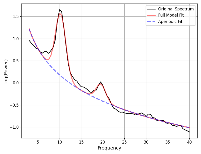
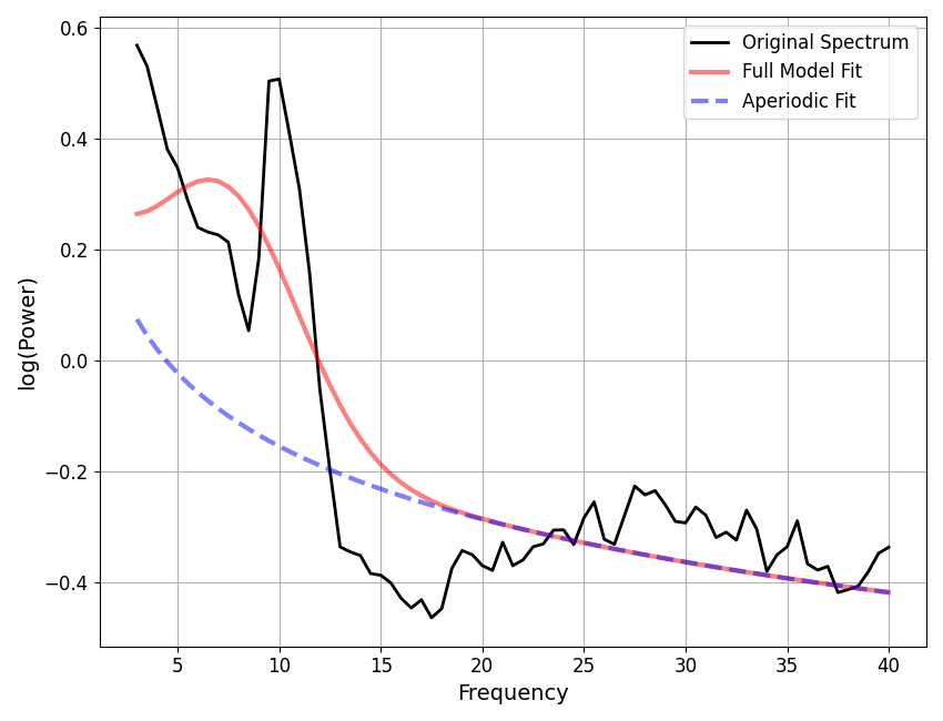
==================================================================================================

                                   FOOOF - POWER SPECTRUM MODEL

                        The model was run on the frequency range 3 - 40 Hz
                                 Frequency Resolution is 0.50 Hz

                            Aperiodic Parameters (offset, exponent):
                                          2.1629, 1.9838

                                       2 peaks were found:
                                CF:  10.24, PW:  1.393, BW:  2.38
                                CF:  19.57, PW:  0.372, BW:  2.19

                                     Goodness of fit metrics:
                                    R^2 of model fit is 0.9891
                                    Error of the fit is 0.0583

==================================================================================================
As a reminder you can save these reports using the .save_report() method, for example, by running fm.save_report(‘INDV_demo’, file_path=output_path).
All of the model fit information is saved to the model object, which we can then access.
Note that all attributes learned in the model fit process have a trailing underscore.
# Access the model fit parameters from the model object
print('Aperiodic parameters: \n', fm.aperiodic_params_, '\n')
print('Peak parameters: \n', fm.peak_params_, '\n')
print('Goodness of fit:')
print('Error - ', fm.error_)
print('R^2   - ', fm.r_squared_, '\n')
print('Number of fit peaks: \n', fm.n_peaks_)
Aperiodic parameters:
 [2.16291607 1.98379651]

Peak parameters:
 [[10.23978577  1.39291114  2.38095481]
 [19.56651381  0.37190896  2.19412328]]

Goodness of fit:
Error -  0.05826562244674064
R^2   -  0.9891330764757991

Number of fit peaks:
 2
Another way to access model fit parameters is to use the get_params method, which can be used to access model fit attributes.
This method can be used to extract periodic and aperiodic parameters.
# Extract aperiodic and periodic parameter
aps = fm.get_params('aperiodic_params')
peaks = fm.get_params('peak_params')
# Extract goodness of fit information
err = fm.get_params('error')
r2s = fm.get_params('r_squared')
# Extract specific parameters
exp = fm.get_params('aperiodic_params', 'exponent')
cfs = fm.get_params('peak_params', 'CF')
# Print out a custom parameter report
template = ("With an error level of {error:1.2f}, specparam fit an exponent "
            "of {exponent:1.2f} and peaks of {cfs:s} Hz.")
print(template.format(error=err, exponent=exp,
                      cfs=' & '.join(map(str, [round(CF, 2) for CF in cfs]))))
With an error level of 0.06, specparam fit an exponent of 1.98 and peaks of 10.24 & 19.57 Hz.
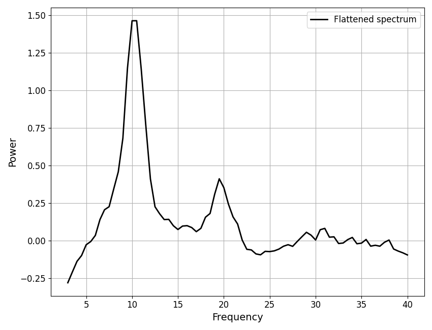
Next, we will plot the flattened power spectrum.
It may be useful to plot a flattened power spectrum, with the aperiodic fit removed.
# Set whether to plot in log-log space
plt_log = False

# Do an initial aperiodic fit - a robust fit, that excludes outliers
init_ap_fit = gen_aperiodic(fm.freqs, fm._robust_ap_fit(fm.freqs, fm.power_spectrum))

# Recompute the flattened spectrum using the initial aperiodic fit
init_flat_spec = fm.power_spectrum - init_ap_fit
# Plot the flattened the power spectrum
plot_spectra(fm.freqs, init_flat_spec, plt_log, label='Flattened spectrum', color='black')
The model object also has I/O utilities for saving and reloading data.
The .save method can be used to save out data from the object, specifying which information to save.
For example, you can save results with the following: - settings: fm.save(‘fit_settings’, save_settings=True, file_path=output_path) - results: `fm.save(‘fit_results’, save_results=True, file_path=output_path) - data: fm.save(‘fit_data’, save_data=True, file_path=output_path)
Another option is to save out data as a .csv rather than the default .json file format. You can do this be exporting the results to a dataframe (see other examples for further guidance on this topic).
# Convert results to dataframe
df = fm.to_df(None)
The above dataframe can be saved out to a csv using the to_csv method.
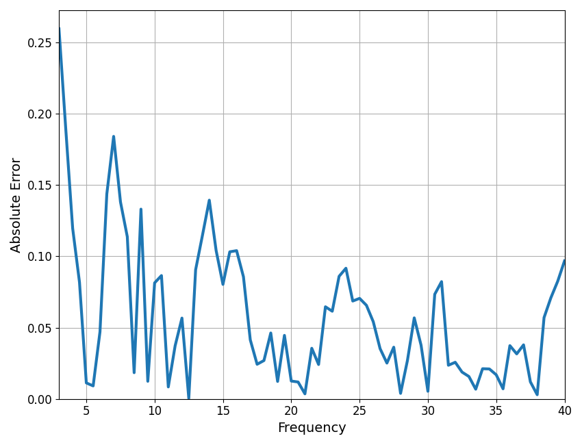
Checking model fit quality
It can be useful to plot frequency-by-frequency error of the model fit, to identify where in frequency space the spectrum is (or is not) being fit well. When fitting individual spectrum, this can be accomplished using the compute_pointwise_error_fm function.
In this case, we can see that error fluctuates around 0.05, which is the same as the mean absolute error for the model (MAE). There are points in the spectrum where the model fit is somewhat poor, particularly < 4 Hz, around 6-9 Hz, and around 14 Hz. Further considerations may be necessary for this model fit.
# Plot frequency-by-frequency error
compute_pointwise_error_fm(fm, plot_errors=True)
# Compute the frequency-by-frequency errors
errs_fm = compute_pointwise_error_fm(fm, plot_errors=False, return_errors=True)
# Note that the average of this error is the same as the global error stored
print('Average freq-by-freq error:\t {:1.3f}'.format(np.mean(errs_fm)))
print('FOOOF model fit error: \t\t {:1.3f}'.format(fm.error_))
Average freq-by-freq error:      0.058
FOOOF model fit error:           0.058
Fitting a Group of Power Spectra
In the next example, we will fit a group of power spectra.
First we need to load the data, including:
freqs.csv, which contains a vector of frequencies
eopPSDs.csv, which contains the power values for a group of power spectrum, one for each subject
# Collect the example data
fetch_fooof_data('freqs.csv', data_path, data_url)
fetch_fooof_data('eop.csv', data_path, data_url)
# Load csv files containing frequency and power values
freqs = np.ravel(pd.read_csv(data_path / "freqs.csv"))
spectra = np.array(pd.read_csv(data_path / "eop.csv"))[:, 1:101]
# Get the number of subjects
n_subjs = spectra.shape[0]
print('There are {:d} subjects.'.format(n_subjs))
There are 60 subjects.
Now we can parameterize our group of power spectra!
# Initialize a model object for spectral parameterization, with some settings
fg = FOOOFGroup(peak_width_limits=peak_width, max_n_peaks=n_peaks,
                min_peak_height=peak_height, verbose=False)

# Fit group PSDs over the 3-40 Hz range
fg.fit(freqs, spectra, PSD_range)
# Print out the group results and plots of fit parameters
fg.print_results()
fg.plot()
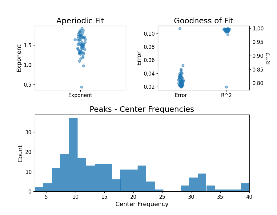
==================================================================================================
FOOOF - GROUP RESULTS
Number of power spectra in the Group: 60
The model was run on the frequency range 3 - 40 Hz
Frequency Resolution is 0.50 Hz
Power spectra were fit without a knee.
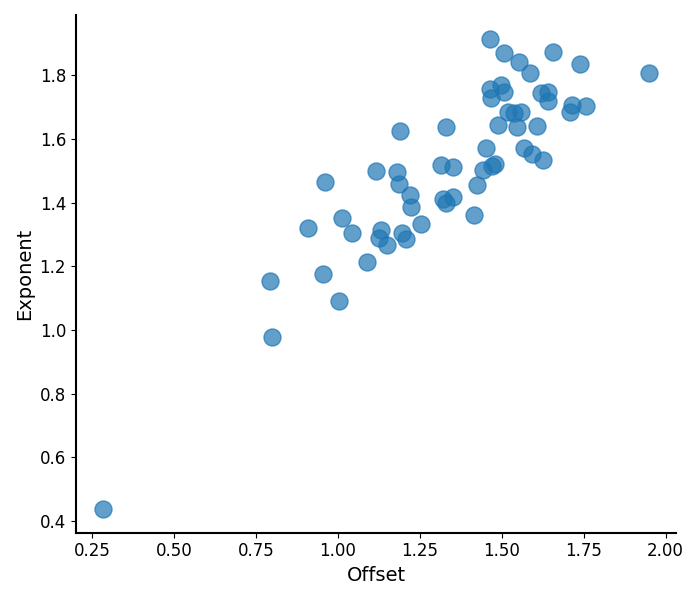
Aperiodic Fit Values:
Exponents - Min: 0.438, Max: 1.915, Mean: 1.515
In total 208 peaks were extracted from the group
Goodness of fit metrics:
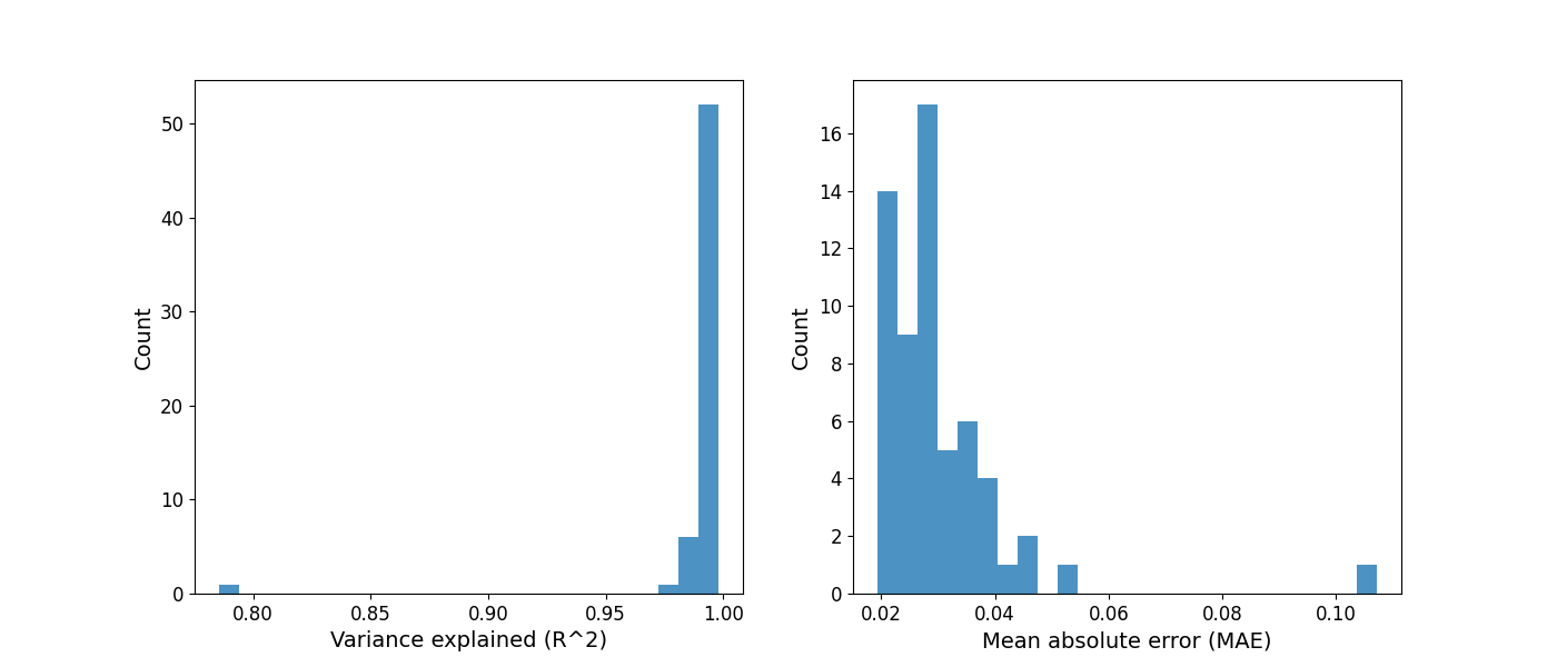
R2s - Min: 0.786, Max: 0.998, Mean: 0.990
Errors - Min: 0.019, Max: 0.107, Mean: 0.030
==================================================================================================
As before, we can also save this report using the .save_report method, for example by calling: fg.save_report(‘EOP_demo’, file_path=output_path).
As with the individual model object, the get_params method can be used to access model fit attributes.
In addition, here we will use a Bands object and the get_band_peak_fg function to organize fit peaks into canonical band ranges.
# Extract aperiodic and full periodic parameters
aps = fg.get_params('aperiodic_params')
per = fg.get_params('peak_params')
# Extract group fit information
err = fg.get_params('error')
r2s = fg.get_params('r_squared')
# Check the average number of fit peaks, per model
print('Average number of fit peaks: ', np.mean(fg.n_peaks_))
Average number of fit peaks: 3.466666666666667
# Extract band-limited peaks information
thetas = get_band_peak_fg(fg, bands.theta)
alphas = get_band_peak_fg(fg, bands.alpha)
betas = get_band_peak_fg(fg, bands.beta)
The specparam module also has functions for plotting the fit parameters.
# Plot the measured aperiodic parameters
plot_aperiodic_params(aps)
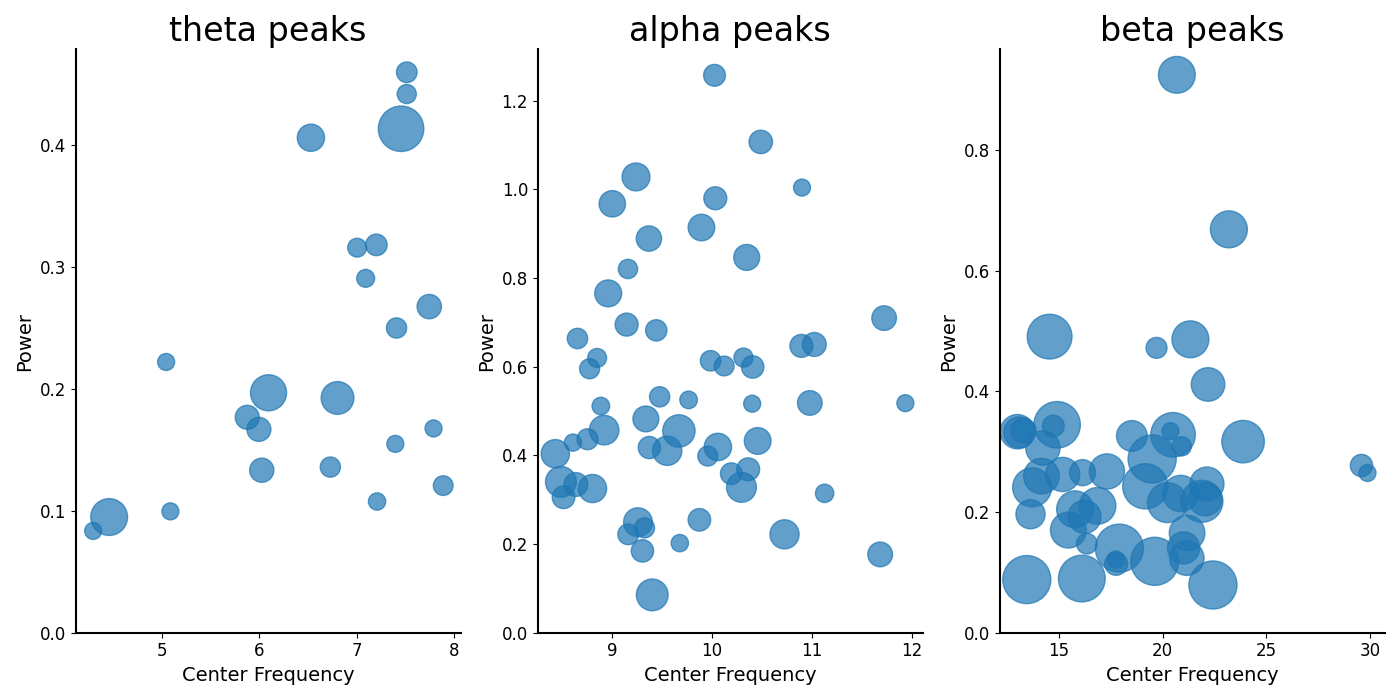
# Plot the parameters for peaks, split up by band
_, axes = plt.subplots(1, 3, figsize=(14, 7))
all_bands = [thetas, alphas, betas]
for ax, label, peaks in zip(np.ravel(axes), bands.labels, all_bands):
    plot_peak_params(peaks, ax=ax)
    ax.set_title(label + ' peaks', fontsize=24)
plt.subplots_adjust(hspace=0.4)
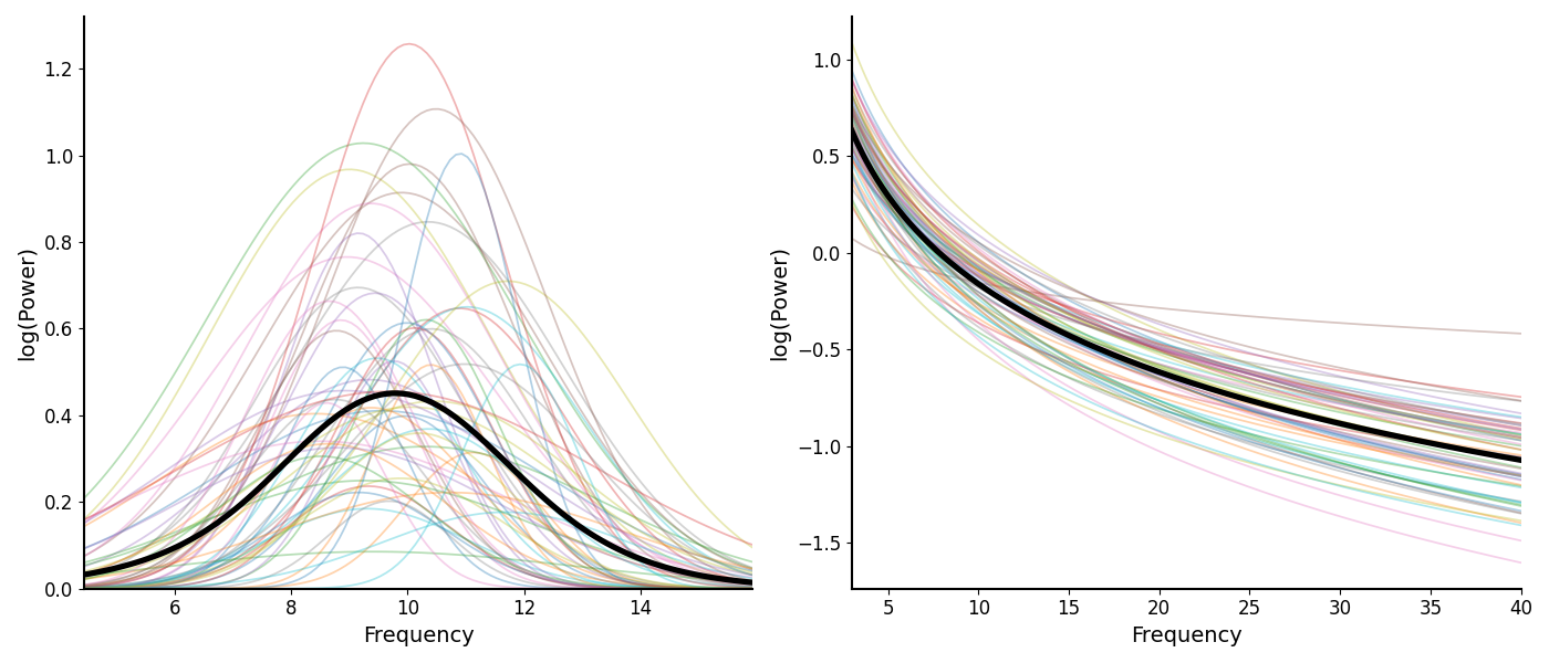
We can also plot reconstructions of model components.
In the following, we plot reconstructed alpha peaks and aperiodic components.
# Plot reconstructions of model components
_, axes = plt.subplots(1, 2, figsize=(14, 6))
plot_peak_fits(alphas, ax=axes[0])
plot_aperiodic_fits(aps, fg.freq_range, ax=axes[1])
Tuning the specparam algorithm
There are no strict guidelines about optimal parameters that will be appropriate across data sets and recording modalities. We suggest applying a data-driven approach to tune model fitting for optimal performance, while taking into account your expectations about periodic and aperiodic activity given the data, the question of interest, and prior findings.
One option is to parameterize a subset of data to evaluate the appropriateness of model fit settings prior to fitting each power spectrum in the data set. Here, we test parameters on a randomly selected 10% of the data. Results are saved out to a Output folder for further consideration.
First, lets randomly sub-sample 10% of the power spectra that we will use to test model settings.
# Set random seed
np.random.seed(1)

# Define settings for & subsample a selection of power spectra
subsample_frac = 0.10
spectra_subsample = subsample_spectra(spectra, subsample_frac)
Here, we first define settings for two models to be fit and compared.
# Define `peak_width_limit` for each model
m1_peak_width = [2, 5]
m2_peak_width = [1, 8]

# Define `max_n_peaks` for each model
m1_n_peaks = 4
m2_n_peaks = 6

# Define `min_peak_height` for each model
m1_peak_height = 0.05
m2_peak_height = 0.10
Next, we set frequency ranges for each model.
To sub-select frequency ranges, we can use the trim_spectrum function to extract frequency ranges of interest for each model.
# Define frequency range for each model
m1_PSD_range = [2, 20]
m2_PSD_range = [3, 40]

# Sub-select frequency ranges
m1_freq, m1_spectra = trim_spectrum(freqs, spectra_subsample, m1_PSD_range)
m2_freq, m2_spectra = trim_spectrum(freqs, spectra_subsample, m2_PSD_range)
Fit models, with different settings.
# Fit model object with model 1 settings
fg1 = FOOOFGroup(peak_width_limits=m1_peak_width, max_n_peaks=m1_n_peaks,
                 min_peak_height=m1_peak_height)
fg1.fit(m1_freq, m1_spectra)

# Create individual reports for model 1 settings (these could be saved and checked)
for ind in range(len(fg1)):
    temp_model = fg1.get_fooof(ind, regenerate=True)
Running FOOOFGroup across 6 power spectra.
We can do the same with the other set of settings.
# Fit model object with model 2 settings
fg2 = FOOOFGroup(peak_width_limits=m2_peak_width, max_n_peaks=m2_n_peaks,
                 min_peak_height=m2_peak_height)
fg2.fit(m2_freq, m2_spectra)

# Create individual reports for model 2 settings (these could be saved and checked)
for ind in range(len(fg2)):
    temp_model = fg2.get_fooof(ind, regenerate=True)
Running FOOOFGroup across 6 power spectra.
There are also other ways to manage settings, for example, using the FOOOFSettings object.
Here we will redefine group model objects (FOOOFGroup), again using different settings for each one.
# Define settings for model 1
settings1 = FOOOFSettings(peak_width_limits=m1_peak_width, max_n_peaks=m1_n_peaks,
                          min_peak_height=m1_peak_height, peak_threshold=2.,
                          aperiodic_mode='fixed')

# Define settings for model 2
settings2 = FOOOFSettings(peak_width_limits=m2_peak_width, max_n_peaks=m2_n_peaks,
                          min_peak_height=m2_peak_height, peak_threshold=2.,
                          aperiodic_mode='fixed')
# Initialize model objects for spectral parameterization, with some settings
fg1 = FOOOFGroup(*settings1)
fg2 = FOOOFGroup(*settings2)
Now, let’s fit models with group model object
Note that when fitting power spectra, you can can specify a fit range to fit the model to, so you don’t have to explicitly trim the spectra.
Here we will refit the example data, specifying the fit range, and then save the group reports.
Running FOOOFGroup across 6 power spectra.
Running FOOOFGroup across 6 power spectra.
At this point, it may typically be useful to save out reports from the above different model fits (using .save_report), such that these different setting regimes can be compared.
After selecting initial model fit settings, and fitting power spectra from the full sample, it is often worthwhile to check the goodness of model fit parameters. Please note, the model objects below correspond to the model fit at the top of this script.
# Plot distributions of goodness of fit parameters
# This information is presented in the print_reports output as well
fig, (ax0, ax1) = plt.subplots(1, 2, figsize=(14, 6))
plot_hist(r2s, label='Variance explained (R^2)', ax=ax0)
plot_hist(err, label='Mean absolute error (MAE)', ax=ax1)
# Find the index of the worst model fit from the group
worst_fit_ind = np.argmax(fg.get_params('error'))

# Extract this model fit from the group
fm = fg.get_fooof(worst_fit_ind, regenerate=True)
# Check results and visualize the extracted model
fm.print_results()
fm.plot()
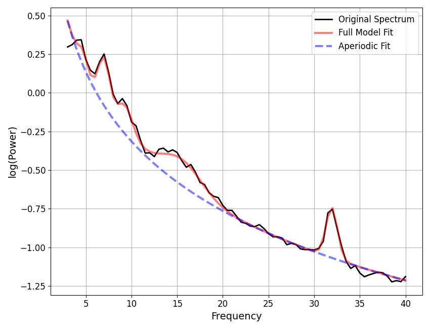
==================================================================================================

                                   FOOOF - POWER SPECTRUM MODEL

                        The model was run on the frequency range 3 - 40 Hz
                                 Frequency Resolution is 0.50 Hz

                            Aperiodic Parameters (offset, exponent):
                                          0.2831, 0.4376

                                       1 peaks were found:
                                CF:   7.45, PW:  0.413, BW:  7.14

                                     Goodness of fit metrics:
                                    R^2 of model fit is 0.7858
                                    Error of the fit is 0.1071

==================================================================================================
Now, let’s check for potential under-fitting.
# Extract all fits that are above some error threshold, for further examination.
underfit_error_threshold = 0.100
underfit_check = []
for ind, res in enumerate(fg):
    if res.error > underfit_error_threshold:
        underfit_check.append(fg.get_fooof(ind, regenerate=True))

Let’s also check for potential over-fitting.
# Extract all fits that are below some error threshold, for further examination.
overfit_error_threshold = 0.02
overfit_check = []
for ind, res in enumerate(fg):
    if res.error < overfit_error_threshold:
        overfit_check.append(fg.get_fooof(ind, regenerate=True))
The same approach for saving out data is available in the group object, using the save method, for example:
settings: fg.save(‘group_settings’, save_settings=True, file_path=output_path)
results: fg.save(‘group_results’, save_results=True, file_path=output_path)
Another option is to export results to a dataframe (from which CSV files can be saved).
# Save out aperiodic parameter results
df = fg.to_df(2)
Frequency-by-frequency errors
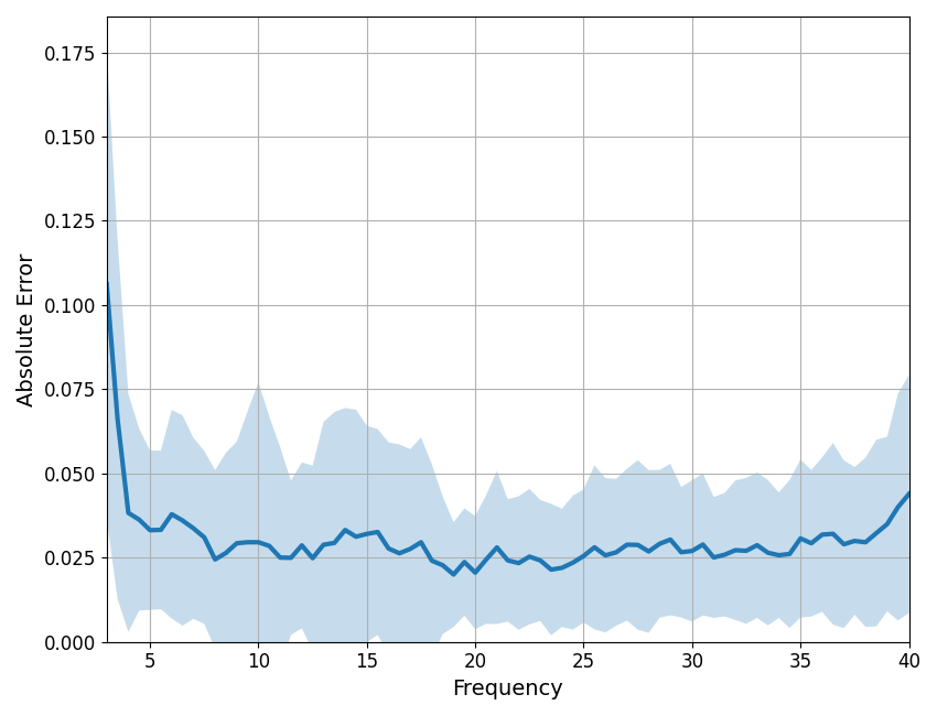
It can be useful to plot frequency-by-frequency error of the model fit, to identify where in frequency space the spectrum is (or is not) being fit well. When fitting individual spectrum, this can be accomplished using the compute_pointwise_error_fg function. When plotting the error, the plot line is the mean error per frequency, across fits, and the shading indicates the standard deviation of the error, also per frequency.
In this case, we can see that error fluctuates around 0.03, which is the same as the mean absolute error for this group fit. There are points in the spectrum where the model fit is somewhat poor, particularly < 4 Hz. The code below lets you identify the highest mean error and largest standard deviation in error for the group fit. In this case, that occurs at 3 Hz, suggesting potential issues with fit at the lower end of the examined frequency range.
# Plot frequency-by-frequency error
compute_pointwise_error_fg(fg, plot_errors=True)
# Return the errors - this returns a 2D matrix of errors for all fits
errs_fg = compute_pointwise_error_fg(fg, plot_errors=False, return_errors=True)

# Check which frequency has the highest error
f_max_err = fg.freqs[np.argmax(np.mean(errs_fg, 0))]
print('Frequency with highest mean error: \t\t\t', f_max_err)

# Check which frequency has the largest standard deviation of error
f_max_std = fg.freqs[np.argmax(np.std(errs_fg, 0))]
print('Frequency with highest standard deviation of error: \t', f_max_std)
Frequency with highest mean error:                       3.0
Frequency with highest standard deviation of error:      3.0
In some cases, it may be necessary to drop poor (or failed) model fits from the group object. This can be done using the fg.drop function, as shown here. In this case, we remove a participant who has a MAE greater than 0.10. The error threshold will vary depending on sample characteristics and data quality.
# Drop poor model fits based on MAE
fg.drop(fg.get_params('error') > 0.10)
Conclusions
For more on this topic, see the DevelopmentalDemo repository and/or the associated paper for further information.
Total running time of the script: (0 minutes 4.428 seconds)