08: Further Analysis

Analyze results from fitting power spectrum models.

Exploring Power Spectrum Model Results

So far we have explored how to parameterize neural power spectra, whereby we can measure parameters of interest from data - in particular measuring aperiodic and periodic activity.

These measured parameters can then be examined within or between groups of interest, and/or fed into further analyses. For example, one could examine if these parameters predict behavioural or physiological features of interest. Largely, it is up to you what to do after fitting power spectrum models, as it depends on your questions of interest.

Here, we briefly introduce some analysis utilities that are included in the module, and explore some simple analyses that can be done with model parameters.

To start, we will load and fit some example data, as well as simulate a group of power spectra to fit with power spectrum models, to use as examples for this tutorial.

# General imports
import numpy as np

# Import the FOOOF and FOOOFGroup objects
from fooof import FOOOF, FOOOFGroup

# Import the Bands object, which is used to define frequency bands
from fooof.bands import Bands

# Import simulation code and utilities
from fooof.sim.params import param_sampler
from fooof.sim.gen import gen_group_power_spectra
from fooof.sim.utils import set_random_seed

# Import some analysis functions
from fooof.analysis import get_band_peak_fm, get_band_peak_fg

# Import a utility to download and load example data
from fooof.utils.download import load_fooof_data

Load and Fit Example Data

First, let’s load and fit an example power spectrum.

# Load example data files needed for this example
freqs = load_fooof_data('freqs.npy', folder='data')
spectrum = load_fooof_data('spectrum.npy', folder='data')

# Fit a power spectrum model
fm = FOOOF(peak_width_limits=[2, 8])
fm.fit(freqs, spectrum, [3, 30])

Simulate and Fit Group Data

We will also simulate and fit some additional example data.

# Set random seed, for consistency generating simulated data
set_random_seed(21)

# Generate some simulated power spectra
freqs, spectra = gen_group_power_spectra(n_spectra=10,
                                         freq_range=[3, 40],
                                         aperiodic_params=param_sampler([[20, 2], [35, 1.5]]),
                                         periodic_params=param_sampler([[], [10, 0.5, 2]]))

# Initialize a FOOOFGroup object with some settings
fg = FOOOFGroup(peak_width_limits=[1, 8], min_peak_height=0.05,
                max_n_peaks=6, verbose=False)

# Fit power spectrum models across the group of simulated power spectra
fg.fit(freqs, spectra)

Analysis Utilities

The FOOOF module includes some analysis functions.

Note that these utilities are generally relatively simple utilities that assist in accessing and investigating the model parameters.

In depth analysis of power spectrum model results is typically idiosyncratic to the goals of the project, and so we consider that this will typically require custom code. Here, we seek to offer the most useful general utilities.

We will demonstrate some of these utility functions covering some general use cases.

Analyzing Periodic Components

We will start by analyzing the periodic components.

These utilities mostly serve to help organize and extract periodic components, for example extracting peaks that fall within defined frequency bands.

This also includes the Bands object, which is a custom, dictionary-like object, that is provided to store frequency band definitions.

# Define frequency bands of interest
bands = Bands({'theta' : [4, 8],
               'alpha' : [8, 12],
               'beta' : [15, 30]})

Extracting peaks from FOOOF Objects

The get_band_peak_fm() function takes in a FOOOF object and extracts peak(s) from a requested frequency range.

You can optionally specify:

• whether to return one peak from the specified band, in which case the highest peak is returned, or whether to return all peaks from within the band

• whether to apply a minimum threshold to extract peaks, for example, to extract peaks only above some minimum power threshold

# Extract any alpha band peaks from the power spectrum model
alpha = get_band_peak_fm(fm, bands.alpha)
print(alpha)

[9.48376672 0.91782115 2.        ]

Extracting peaks from FOOOFGroup Objects

Similarly, the get_band_peak_fg() function can be used to select peaks from specified frequency ranges, from FOOOFGroup objects.

Note that you can also apply a threshold to extract group peaks but, as discussed below, this approach will always only extract at most one peak per individual model fit from the FOOOFGroup object.

# Get all alpha peaks from a group of power spectrum models
alphas = get_band_peak_fg(fg, bands.alpha)

# Check out some of the alpha parameters
print(alphas[0:5, :])

[[10.03970097  0.48627814  3.78823186]
 [10.03394843  0.48807386  3.82620803]
 [        nan         nan         nan]
 [10.04095697  0.49087309  3.81808357]
 [        nan         nan         nan]]

When selecting peaks from a group of model fits, we want to retain information about which model each peak comes from.

To do so, the output of get_band_peak_fg() is organized such that each row corresponds to a specific model fit. This means that returned array has the shape [n_models, 3], and so the index of each row corresponds to the index of the model from the FOOOFGroup object.

For this to work, at most 1 peak is extracted for each model fit within the specified band. If more than 1 peak are found within the band, the peak with the highest power is extracted. If no peaks are found, that row is filled with ‘nan’.

# Check descriptive statistics of extracted peak parameters
print('Alpha CF : {:1.2f}'.format(np.nanmean(alphas[:, 0])))
print('Alpha PW : {:1.2f}'.format(np.nanmean(alphas[:, 1])))
print('Alpha BW : {:1.2f}'.format(np.nanmean(alphas[:, 2])))

Alpha CF : 10.03
Alpha PW : 0.49
Alpha BW : 3.81

Customizing Peak Extraction

If you want to do more customized extraction of peaks, for example, extracting all peaks in a frequency band from each model in a FOOOFGroup object, you may need to use the underlying functions that operate on arrays of peak parameters. To explore these functions, check the listings in the API page.

A Note on Frequency Ranges

A benefit of fitting power spectrum models is that you do not have to define a priori frequency ranges from which to extract peaks.

Nevertheless, it may still be useful to group extracted peaks into ‘bands’ of interest, which is why the aforementioned functions are offered.

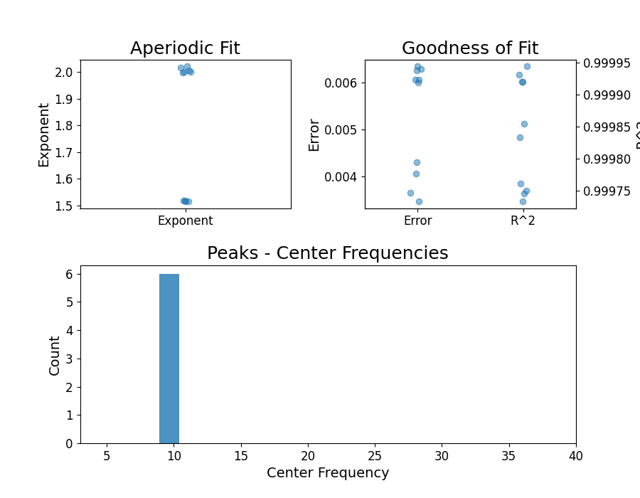
Since this frequency-range selection can be done after model fitting, we do recommend checking the model results, for example by checking a histogram of the center frequencies extracted across a group, in order to ensure the frequency ranges you choose reflect the characteristics of the data under study.

Analyzing the Aperiodic Component

Typically, for analyzing the aperiodic component of the data, aperiodic parameters just need to be extracted from FOOOF objects and fit into analyses of interest.

# Plot from the FOOOFGroup, to visualize the parameters
fg.plot()

# Extract aperiodic exponent parameters from group results
exps = fg.get_params('aperiodic_params', 'exponent')

# Check out the aperiodic exponent results
print(exps)

[1.5174828  1.51806721 1.99827884 1.5156351  2.00559925 2.01700246
 2.00089211 2.02010985 1.51575182 1.99955831]

Example Analyses

Once you have extracted parameters of interest, you can analyze them by, for example:

• Characterizing periodic & aperiodic properties, and analyzing spatial topographies, across demographics, modalities, and tasks

• Comparing peaks within and between subjects across different tasks of interest

• Predicting disease state based on power spectrum model parameters

• Fitting power spectrum models in a trial-by-trial approach to try and decode task properties, and behavioral states

So far we have only introduced the basic utilities to help with selecting and examining power spectrum model parameters.

To further explore some of these specific analyses, and explore other utilities that may be useful, check out the examples page.

Conclusion

This is the end of the main tutorial materials!

If you are having any troubles, please submit an issue on Github here.