Note
Go to the end to download the full example code.
07: Tuning & Troubleshooting
Tips & tricks for choosing algorithm settings, tuning fits, and troubleshooting.
# General imports
import numpy as np

# Import the FOOOF and FOOOFGroup objects
from fooof import FOOOF, FOOOFGroup

# Import some utilities for creating simulated power-spectra
from fooof.sim.params import param_sampler
from fooof.sim.gen import gen_power_spectrum, gen_group_power_spectra
from fooof.sim.utils import set_random_seed
Algorithm Settings
With default settings, the power spectrum model is relatively minimally constrained. It defaults as such since there are not universal settings that work across all different recording modalities. Appropriate settings also vary with power spectrum quality (noise, or effectively, the smoothness of the power spectrum), and frequency ranges.
For any given dataset, you will likely have to tune some of the algorithm settings for optimal performance.
To do so, we suggest using a combination of the following considerations:
A priori constraints, given your data, such as the number of peaks you expect to extract
Qualitative analysis, guided by examining the the plotted model fit results, as compared to input data
Quantitative analysis, considering the model goodness of fit metrics (however, see note at the bottom regarding interpreting these metrics)
Choosing settings to tune model fitting is an imperfect art, and should be done carefully, as assumptions built into the settings chosen will impact the model results. Model fitting is generally not overly sensitive to small changes in the settings, so as long as broadly appropriate settings are chosen, small perturbations to these chosen settings should not have a large impact on the fitting.
We do recommend that model settings should not be changed between power spectra (across channels, trials, or subjects), if they are to be meaningfully compared. We therefore recommend first testing fitting the model across some representative spectra, in order to select settings, which you then keep constant for the full analysis.
Tuning the Algorithm
With default settings, the model fit is fairly liberal at fitting peaks, and so most commonly this will lead to overfitting, being overzealous at fitting small noisy bumps as peaks.
In some cases, you may also find you need to relax some settings, to get better fits.
You also need to make sure you pick an appropriate aperiodic fitting procedure, and that your data meets the assumptions of the approach you choose (see the tutorial on aperiodic fitting).
The remainder of this notebook goes through some examples of choosing settings for different datasets.
Interpreting Model Fit Quality Measures
After model fitting, some goodness of fit metrics are calculated to assist with assessing
the quality of the model fits. It calculates both the model fit error, as the mean absolute
error (MAE) between the full model fit (fooofed_spectrum_) and the original power spectrum,
as well as the R-squared correspondence between the original spectrum and the full model.
These scores can be used to assess how the model is performing. However interpreting these measures requires a bit of nuance. Model fitting is NOT optimized to minimize fit error / maximize r-squared at all costs. To do so typically results in fitting a large number of peaks, in a way that overfits noise, and only artificially reduces error / maximizes r-squared.
The power spectrum model is therefore tuned to try and measure the aperiodic component and peaks in a parsimonious manner, and, fit the right model (meaning the right aperiodic component and the right number of peaks) rather than the model with the lowest error.
Given this, while high error / low r-squared may indicate a poor model fit, very low error / high r-squared may also indicate a power spectrum that is overfit, in particular in which the peak parameters from the model may reflect overfitting by fitting too many peaks.
We therefore recommend that, for a given dataset, initial explorations should involve checking both cases in which model fit error is particularly large, as well as when it is particularly low. These explorations can be used to pick settings that are suitable for running across a group. There are not universal settings that optimize this, and so it is left up to the user to choose settings appropriately to not under- or over-fit for a given modality / dataset / application.
Reducing Overfitting
If the model appears to be overfitting (for example, fitting too many peaks to small bumps), try:
Setting a lower-bound bandwidth-limit, to exclude fitting very narrow peaks, that may be noise
Setting a maximum number of peaks that the algorithm may fit: max_n_peaks
If set, the algorithm will fit (up to) the max_n_peaks highest power peaks.
Setting a minimum absolute peak height: min_peak_height
Simulating Power Spectra
For this example, we will use simulated data. The FOOOF module includes utilities
for creating simulated power-spectra. To do so, we can use the gen_power_spectrum()
function to simulate individual power spectra, following the power spectrum model.
First, we will start by generating a noisy simulated power spectrum
# Set the frequency range to generate the power spectrum
f_range = [1, 50]
# Set aperiodic component parameters, as [offset, exponent]
ap_params = [20, 2]
# Gaussian peak parameters
gauss_params = [[10, 1.0, 2.5], [20, 0.8, 2], [32, 0.6, 1]]
# Set the level of noise to generate the power spectrum with
nlv = 0.1

# Set random seed, for consistency generating simulated data
set_random_seed(21)

# Create a simulated power spectrum
freqs, spectrum = gen_power_spectrum(f_range, ap_params, gauss_params, nlv)
FOOOF WARNING: Lower-bound peak width limit is < or ~= the frequency resolution: 0.50 <= 0.50
Lower bounds below frequency-resolution have no effect (effective lower bound is the frequency resolution).
Too low a limit may lead to overfitting noise as small bandwidth peaks.
We recommend a lower bound of approximately 2x the frequency resolution.
==================================================================================================
FOOOF - POWER SPECTRUM MODEL
The model was run on the frequency range 1 - 50 Hz
Frequency Resolution is 0.50 Hz
Aperiodic Parameters (offset, exponent):
20.0456, 2.0236
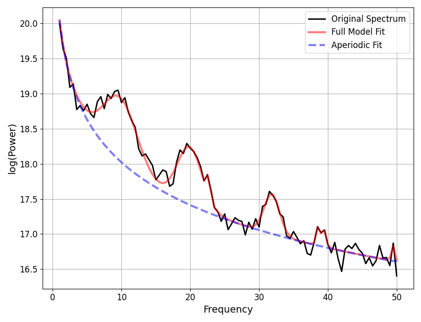
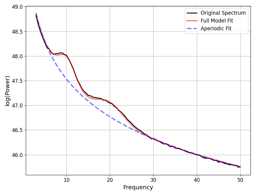
7 peaks were found:
CF: 9.83, PW: 0.908, BW: 4.90
CF: 19.92, PW: 0.826, BW: 3.60
CF: 22.69, PW: 0.525, BW: 0.50
CF: 31.85, PW: 0.566, BW: 2.22
CF: 38.65, PW: 0.262, BW: 0.59
CF: 39.50, PW: 0.239, BW: 0.54
CF: 49.46, PW: 0.209, BW: 0.50
Goodness of fit metrics:
R^2 of model fit is 0.9893
Error of the fit is 0.0710
==================================================================================================
Notice that in the above fit, we are very likely to think that the model has been overzealous in fitting peaks, and is therefore overfitting.
This is also suggested by the model r-squared, which is suspiciously high, given the amount of noise we in the simulated power spectrum.
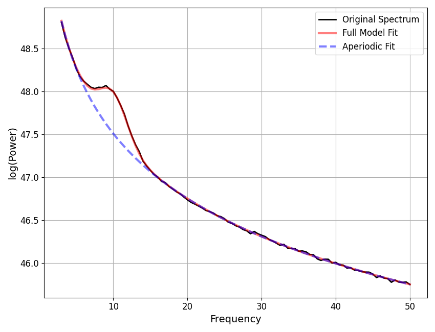
To reduce this kind of overfitting, we can update the algorithm settings.
==================================================================================================
FOOOF - POWER SPECTRUM MODEL
The model was run on the frequency range 1 - 50 Hz
Frequency Resolution is 0.50 Hz
Aperiodic Parameters (offset, exponent):
20.0242, 1.9996
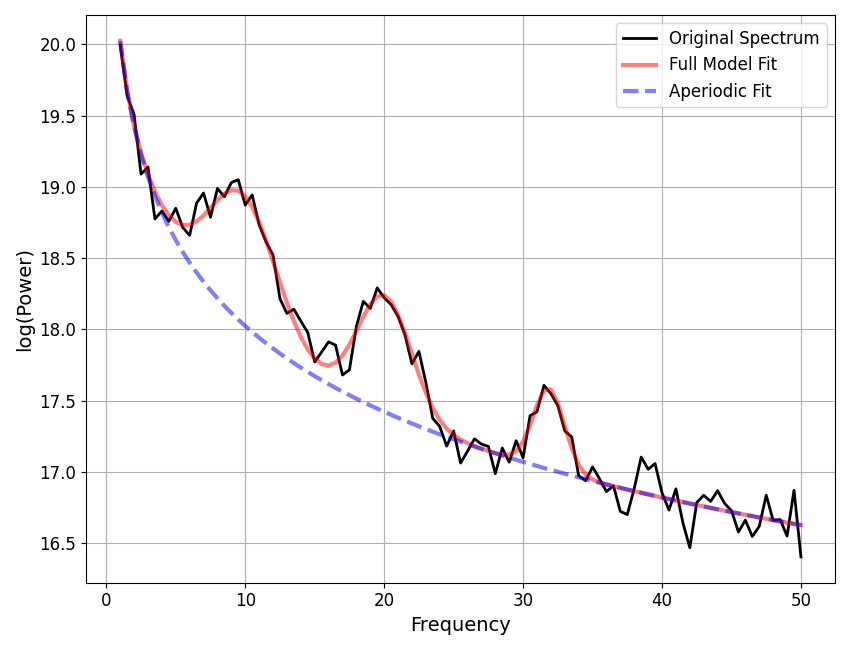
3 peaks were found:
CF: 9.82, PW: 0.910, BW: 4.87
CF: 20.03, PW: 0.817, BW: 3.88
CF: 31.85, PW: 0.566, BW: 2.22
Goodness of fit metrics:
R^2 of model fit is 0.9860
Error of the fit is 0.0823
==================================================================================================
We can compare how the model fit, using the updated settings, compares to the ground truth of the simulated spectrum.
Note that the simulation parameters are defined in terms of Gaussian parameters, which are slightly different from the peak parameters (see the note in tutorial 02), which is why we compare to the model gaussian parameters here.
# Compare ground truth simulated parameters to model fit results
print('Ground Truth \t\t Model Parameters')
for sy, fi in zip(np.array(gauss_params), fm.gaussian_params_):
    print('{:5.2f} {:5.2f} {:5.2f} \t {:5.2f} {:5.2f} {:5.2f}'.format(*sy, *fi))
Ground Truth             Model Parameters
10.00  1.00  2.50         9.82  0.91  2.43
20.00  0.80  2.00        20.03  0.82  1.94
32.00  0.60  1.00        31.85  0.57  1.11
Power Spectra with No Peaks
A known case in which the model can overfit is in power spectra in which no peaks are
present. In this case, the standard deviation can be very low, and so the relative
peak height check (min_peak_threshold) is very liberal at keeping gaussian fits.
If you expect, or know, you have power spectra without peaks in your data,
we recommend using the min_peak_height setting. Otherwise, the model is unlikely to
appropriately fit power spectra as having no peaks, since it uses only a relative
threshold if min_peak_height is set to zero (which is the default value).
Setting min_peak_height requires checking the scale of your power spectra,
allowing you to define an absolute threshold for extracting peaks.
Reducing Underfitting
If you are finding that the model is underfitting:
First check and perhaps loosen any restrictions from
max_n_peaksandmin_peak_heightTry updating
peak_thresholdto a lower valueBad fits may stem from issues with aperiodic component fitting
Double check that you are using the appropriate aperiodic mode
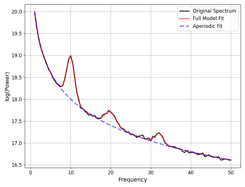
Next we will simulate a much smoother power spectrum, and update settings accordingly.
# Set the frequency range to generate the power spectrum
f_range = [1, 50]
# Define aperiodic parameters, as [offset, exponent]
ap_params = [20, 2]
# Define peak parameters, each peak defined as [CF, PW, BW]
gauss_params = [[10, 1.0, 1.0], [20, 0.3, 1.5], [32, 0.25, 1]]
# Set the level of noise to generate the power spectrum with
nlv = 0.025

# Create a simulated power spectrum
freqs, spectrum = gen_power_spectrum([1, 50], ap_params, gauss_params, nlv=nlv)
==================================================================================================

                                   FOOOF - POWER SPECTRUM MODEL

                        The model was run on the frequency range 1 - 50 Hz
                                 Frequency Resolution is 0.50 Hz

                            Aperiodic Parameters (offset, exponent):
                                         19.9965, 1.9965

                                       3 peaks were found:
                                CF:  10.00, PW:  0.986, BW:  1.94
                                CF:  19.95, PW:  0.310, BW:  2.78
                                CF:  32.04, PW:  0.231, BW:  1.97

                                     Goodness of fit metrics:
                                    R^2 of model fit is 0.9992
                                    Error of the fit is 0.0182

==================================================================================================
# Check reconstructed parameters compared to the simulated parameters
print('Ground Truth \t\t Model Parameters')
for sy, fi in zip(np.array(gauss_params), fm.gaussian_params_):
    print('{:5.2f} {:5.2f} {:5.2f} \t {:5.2f} {:5.2f} {:5.2f}'.format(*sy, *fi))
Ground Truth             Model Parameters
10.00  1.00  1.00        10.00  0.99  0.97
20.00  0.30  1.50        19.95  0.31  1.39
32.00  0.25  1.00        32.04  0.23  0.98
Checking Fits Across a Group
So far we have explored troubleshooting individual model fits. When starting a new analysis, or working with a new dataset, we do recommend starting by trying some individual fits like this.
If and when you move to using FOOOFGroup to fit groups of power spectra,
there are some slightly different ways to investigate groups of fits,
which we’ll step through now, using some simulated data.
Simulating a Group of Power Spectra
We will continue using simulated data, this time simulating a group of power spectra.
To simulate a group of power spectra, we will use the gen_group_power_spectra()
in combination with called param_sampler() that is used to sample across
possible parameters.
For more and descriptions and example of how the simulations work, check out the examples section.
# Simulation settings for a group of power spectra
n_spectra = 10
sim_freq_range = [3, 50]
nlv = 0.010

# Set the parameter options for aperiodic component and peaks
ap_opts = param_sampler([[20, 2], [50, 2.5], [35, 1.5]])
gauss_opts = param_sampler([[], [10, 0.5, 2], [10, 0.5, 2, 20, 0.3, 4]])

# Simulate a group of power spectra
freqs, power_spectra = gen_group_power_spectra(n_spectra, sim_freq_range,
                                               ap_opts, gauss_opts, nlv)
# Initialize a FOOOFGroup object
fg = FOOOFGroup(peak_width_limits=[1, 6])
# Fit power spectrum models and report on the group
fg.report(freqs, power_spectra)
Running FOOOFGroup across 10 power spectra.
==================================================================================================
FOOOF - GROUP RESULTS
Number of power spectra in the Group: 10
The model was run on the frequency range 3 - 50 Hz
Frequency Resolution is 0.50 Hz
Power spectra were fit without a knee.
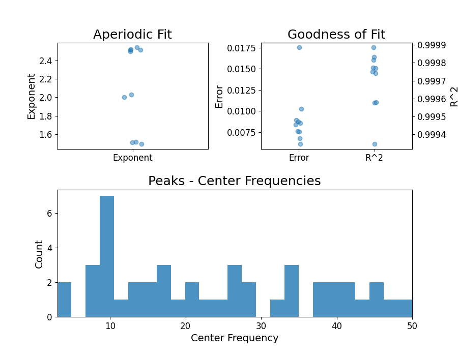
Aperiodic Fit Values:
Exponents - Min: 1.495, Max: 2.539, Mean: 2.114
In total 45 peaks were extracted from the group
Goodness of fit metrics:
R2s - Min: 0.999, Max: 1.000, Mean: 1.000
Errors - Min: 0.006, Max: 0.018, Mean: 0.009
==================================================================================================
In the FOOOFGroup report we can get a sense of the overall performance
by looking at the information about the goodness of fit metrics, and also things like
the distribution of peaks.
However, while these metrics can help identify if fits are, on average, going well (or not) they don’t necessarily indicate the source of any problems.
To do so, we will typically still want to visualize some example fits, to see
what is happening. To do so, next we will find which fits have the most error,
and select these fits from the FOOOFGroup object to visualize.
# Find the index of the worst model fit from the group
worst_fit_ind = np.argmax(fg.get_params('error'))

# Extract this model fit from the group
fm = fg.get_fooof(worst_fit_ind, regenerate=True)
# Check results and visualize the extracted model
fm.print_results()
fm.plot()
==================================================================================================

                                   FOOOF - POWER SPECTRUM MODEL

                        The model was run on the frequency range 3 - 50 Hz
                                 Frequency Resolution is 0.50 Hz

                            Aperiodic Parameters (offset, exponent):
                                         50.0718, 2.5387

                                       2 peaks were found:
                                CF:  10.18, PW:  0.466, BW:  3.80
                                CF:  20.08, PW:  0.300, BW:  6.00

                                     Goodness of fit metrics:
                                    R^2 of model fit is 0.9993
                                    Error of the fit is 0.0175

==================================================================================================
You can also loop through all the results in a FOOOFGroup, extracting
all fits that meet some criterion that makes them worth checking.
This might be checking for fits above some error threshold, as below, but note that you may also want to do a similar procedure to examine fits with the lowest error, to check if the model may be overfitting, or perhaps fits with a particularly large number of gaussians.
# Extract all fits that are above some error threshold, for further examination.
#  You could also do a similar analysis for particularly low errors
error_threshold = 0.010
to_check = []
for ind, res in enumerate(fg):
    if res.error > error_threshold:
        to_check.append(fg.get_fooof(ind, regenerate=True))

# A more condensed version of the procedure above can be written like this:
#to_check = [fg.get_fooof(ind, True) for ind, res in enumerate(fg) if res.error > error_threshold]
# Loop through the problem fits, checking the plots, and saving out reports, to check later.
for ind, fm in enumerate(to_check):
    fm.plot()
    fm.save_report('Report_ToCheck_#' + str(ind))

/Users/tom/opt/anaconda3/lib/python3.8/site-packages/fooof/core/reports.py:72: UserWarning: This figure includes Axes that are not compatible with tight_layout, so results might be incorrect.
  plt.savefig(fpath(file_path, fname(file_name, SAVE_FORMAT)))
/Users/tom/opt/anaconda3/lib/python3.8/site-packages/fooof/core/reports.py:72: UserWarning: This figure includes Axes that are not compatible with tight_layout, so results might be incorrect.
  plt.savefig(fpath(file_path, fname(file_name, SAVE_FORMAT)))
/Users/tom/opt/anaconda3/lib/python3.8/site-packages/fooof/core/reports.py:72: UserWarning: This figure includes Axes that are not compatible with tight_layout, so results might be incorrect.
  plt.savefig(fpath(file_path, fname(file_name, SAVE_FORMAT)))
/Users/tom/opt/anaconda3/lib/python3.8/site-packages/fooof/core/reports.py:72: UserWarning: This figure includes Axes that are not compatible with tight_layout, so results might be incorrect.
  plt.savefig(fpath(file_path, fname(file_name, SAVE_FORMAT)))
Another thing that can be worth keeping an eye on is the average number of fit peaks per model. A particularly high value can indicate overfitting.
# Check the average number of fit peaks, per model
print('Average number of fit peaks: ', np.mean(fg.n_peaks_))
Average number of fit peaks: 4.5
Reporting Bad Fits
If, after working through these suggestions, you are still getting bad fits, and/or are just not sure what is going on, please get in touch! We will hopefully be able to make further recommendations, and this also serves as a way for us to investigate when and why model fitting fails, so that we can continue to make it better.
You can report issues on Github here <https://github.com/fooof-tools/fooof>.
There is also a helper method to print out instructions for reporting bad fits / bugs back to us, as demonstrated below.
# Print out instructions to report bad fits
#  Note you can also call this from FOOOFGroup, and from instances (ex: `fm.print_report_issue()`)
FOOOF.print_report_issue()
==================================================================================================

                                     FOOOF - ISSUE REPORTING

                      Please report any bugs or unexpected errors on Github.
                           https://github.com/fooof-tools/fooof/issues

                   If FOOOF gives you any weird / bad fits, please let us know!
                    To do so, send us a FOOOF report, and a FOOOF data file,

               With a FOOOF object (fm), after fitting, run the following commands:
                             fm.create_report('FOOOF_bad_fit_report')
                         fm.save('FOOOF_bad_fit_data', True, True, True)

                                 Send the generated files to us.
                      We will have a look, and provide any feedback we can.

                            Contact address: voytekresearch@gmail.com

==================================================================================================
Conclusion
We have now stepped through the full work-flow of fitting power spectrum models, using FOOOF objects, picking settings, and troubleshooting model fits. In the next and final tutorial, we will introduce how to start analyzing FOOOF results.
Total running time of the script: (0 minutes 3.095 seconds)