Transforming Power Spectra

Apply transformations to power spectra.

One of the goals of parameterizing neural power spectra is to be able to understand if and how power spectra may be different and/or be changing across time or context.

In order to explore how power spectra can change, the simulation framework also provides functions and utilities for transforming power spectra. These approaches can be useful to specifically define changes and how spectra relate to each other, and track how outcome measures relate to changes in the power spectra.

import numpy as np
import matplotlib.pyplot as plt

# Import the FOOOF object
from fooof import FOOOF

# Import simulation utilities to create example data
from fooof.sim.gen import gen_power_spectrum

# Import functions that can transform power spectra
from fooof.sim.transform import (rotate_spectrum, translate_spectrum,
                                 rotate_sim_spectrum, translate_sim_spectrum,
                                 compute_rotation_offset, compute_rotation_frequency)

# Import plot function to visualize power spectra
from fooof.plts.spectra import plot_spectra

# Generate a simulated power spectrum
freqs, powers, params = gen_power_spectrum([3, 40], [1, 1], [10, 0.5, 1],
                                           return_params=True)

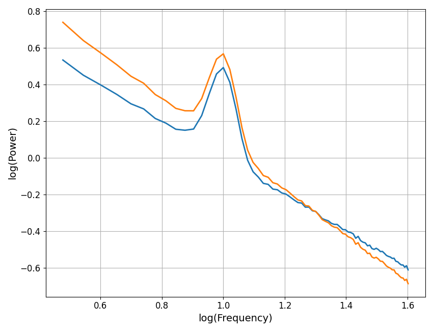
Rotating Power Spectra

The rotate_spectrum() function takes in a power spectrum, and rotates the power spectrum a specified amount, around a specified frequency point, changing the aperiodic exponent of the spectrum.

# Rotation settings
delta_exp = 0.25        # How much to change the exponent by
f_rotation = 20         # The frequency at which to rotate the spectrum

# Rotate the power spectrum
r_powers = rotate_spectrum(freqs, powers, delta_exp, f_rotation)

# Plot the two power spectra, with the rotation applied
plot_spectra(freqs, [powers, r_powers], log_freqs=True, log_powers=True)

Next, we can fit power spectrum models to check if our change in exponent worked as expected.

# Initialize FOOOF objects
fm1 = FOOOF(verbose=False)
fm2 = FOOOF(verbose=False)

# Fit power spectrum models to the original, and rotated, spectrum
fm1.fit(freqs, powers)
fm2.fit(freqs, r_powers)

# Check the measured exponent values
print("Original exponent value:\t {:1.2f}".format(\
    fm1.get_params('aperiodic_params', 'exponent')))
print("Rotated exponent value:\t{:1.2f}".format(\
    fm2.get_params('aperiodic_params', 'exponent')))

Original exponent value:         1.00
Rotated exponent value: 1.25

Rotation Related Offset Changes

Note that when you rotate a power spectrum, the offset also necessarily changes.

If you wish to compute the change in offset that occurs due to a change in exponent, you can use the compute_rotation_offset() function.

# Calculate the change in offset from an exponent change
off_change = compute_rotation_offset(delta_exp, f_rotation)

# Check the change in offset
print("The induced change in offset is: \t {:1.2f}".format(off_change))

The induced change in offset is:         0.33

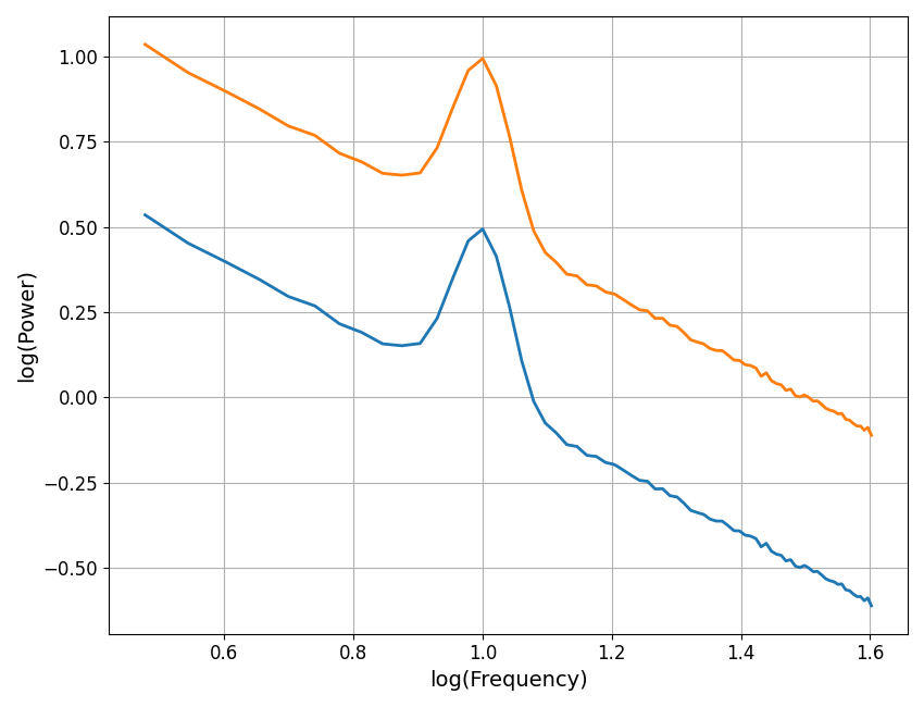
Translating Power Spectra

Another transformation you can apply to power spectra is a translation, which changes the offset, effectively moving the whole spectrum up or down.

Note that changing the offset does not change the exponent.

# Translation settings
delta_offset = 0.5        # How much to change the offset by

# Translate the power spectrum
t_powers = translate_spectrum(powers, delta_offset)

# Plot the two power spectra, with the translation applied
plot_spectra(freqs, [powers, t_powers], log_freqs=True, log_powers=True)

Transforming while Tracking Simulation Parameters

As we’ve seen, transforming power spectra changes their definitions, and sometimes more than just the parameter we are manipulating directly.

If you are transforming simulated spectra, it can be useful to keep track of these changes.

To do so, there are also the functions rotate_sim_spectrum() and translate_sim_spectrum(), which work the same as what we’ve seen so far, with the addition that they take in a SimParams object, and update and return a new SimParams object that tracks the updated simulation parameters.

# Rotate a power spectrum, tracking and updating simulation parameters
r_s_powers, r_params = rotate_sim_spectrum(freqs, powers, delta_exp, f_rotation, params)

# Check the updated sim params from after the rotation
print(r_params)

SimParams(aperiodic_params=[1.3252574989159953, 1.25], periodic_params=[[10, 0.5, 1]], nlv=0.005)

# Translate a power spectrum, tracking and updating simulation parameters
t_s_powers, t_params = translate_sim_spectrum(powers, delta_offset, params)

# Check the updated sim params from after the translation
print(t_params)

SimParams(aperiodic_params=[1.5, 1], periodic_params=[[10, 0.5, 1]], nlv=0.005)

Relations Between Power Spectra

In some cases, what we care about when transforming power spectra, is the relation between multiple transformed power spectra.

For example, if we start with a power spectrum ‘A’, and compute two transformations on it, call them ‘B’ and ‘C’ at the same or different changes in exponent and/or rotation frequencies, what is the relation between ‘B’ and ‘C’?

In the following examples, we will explore the relations between transformed power spectra.

# Create a baseline power spectrum
freqs, powers = gen_power_spectrum([3, 50], [0, 1.5], [10, 0.3, 0.5], nlv=0)

# Initialize some power spectrum models for checking our transformations
fm1 = FOOOF(verbose=False)
fm2 = FOOOF(verbose=False)

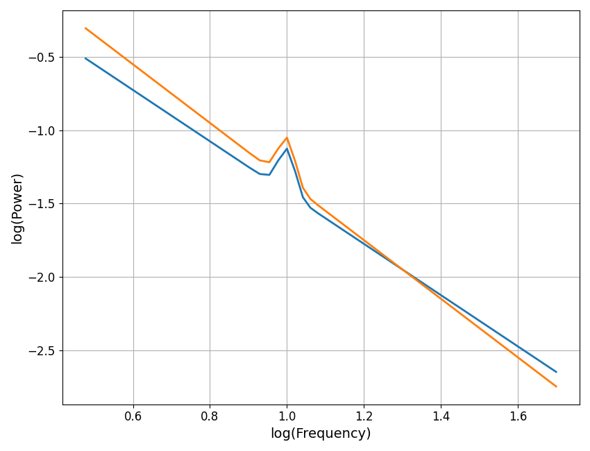
Rotate at the Same Rotation Frequencies

First, let’s consider the case in which we rotate a spectrum by the different delta exponents, at the same rotation frequency.

In this case, each rotation creates the same change in offset between ‘B’ & ‘C’, and so B & C end up with the same offset. The difference in exponent between ‘B’ and ‘C’ is computable as the different of delta exponents applied to each spectrum.

# Settings for rotating power spectra
delta_exp_1 = 0.25
delta_exp_2 = 0.5
f_rotation = 20

# Rotate a spectrum, different amounts, at the same rotation frequency
powers_1 = rotate_spectrum(freqs, powers, delta_exp_1, f_rotation)
powers_2 = rotate_spectrum(freqs, powers, delta_exp_2, f_rotation)

# Calculate the expected difference in exponent
exp_diff = delta_exp_1 - delta_exp_2

# Calculate the measured difference in exponent
fm1.fit(freqs, powers_1); fm2.fit(freqs, powers_2)
exp_diff_meas = fm1.get_params('aperiodic', 'exponent') - \
    fm2.get_params('aperiodic', 'exponent')

# Print out the expected and measured changes in exponent
template = "Exponent Difference: \n  expected: \t{:1.4f} \n  actual: \t{:1.4f}"
print(template.format(exp_diff, exp_diff_meas))

Exponent Difference:
  expected:     -0.2500
  actual:       -0.2500

# Visualize the transformed power spectra
plot_spectra(freqs, [powers_1, powers_2],
             log_freqs=True, log_powers=True)

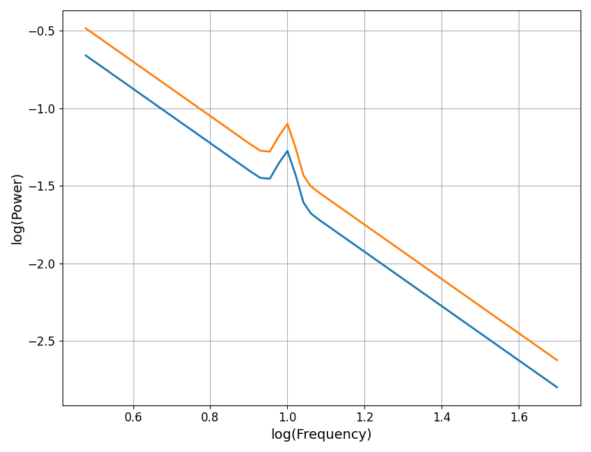
Rotate at Different Rotation Frequencies

Next, let’s consider the case in which we rotate a spectrum by the same delta exponent, but do so at different rotation frequencies.

The resulting power spectra will have the same final exponent value, but there will be a difference in offset between them, as each rotation, at different rotation points, creates a different change in offset. The difference in offset between ‘B’ & ‘C’ is computed as the difference of rotation offset changes between them.

# Settings for rotating power spectra
delta_exp = 0.25
f_rotation_1 = 5
f_rotation_2 = 25

# Rotate a spectrum, the same amount, at two different rotation frequencies
powers_1 = rotate_spectrum(freqs, powers, delta_exp, f_rotation_1)
powers_2 = rotate_spectrum(freqs, powers, delta_exp, f_rotation_2)

# Calculate the expected difference in offset
off_diff = compute_rotation_offset(delta_exp, f_rotation_1) - \
    compute_rotation_offset(delta_exp, f_rotation_2)

# Calculate the measured difference in offset
fm1.fit(freqs, powers_1)
fm2.fit(freqs, powers_2)
off_diff_2 = fm1.get_params('aperiodic', 'offset') - \
    fm2.get_params('aperiodic', 'offset')

# Print out the expected and measured changes in offset
template = "Offset Difference: \n  expected: \t{:1.4f} \n  actual: \t{:1.4f}"
print(template.format(off_diff, off_diff_2))

Offset Difference:
  expected:     -0.1747
  actual:       -0.1747

# Visualize the transformed power spectra
plot_spectra(freqs, [powers_1, powers_2],
             log_freqs=True, log_powers=True)

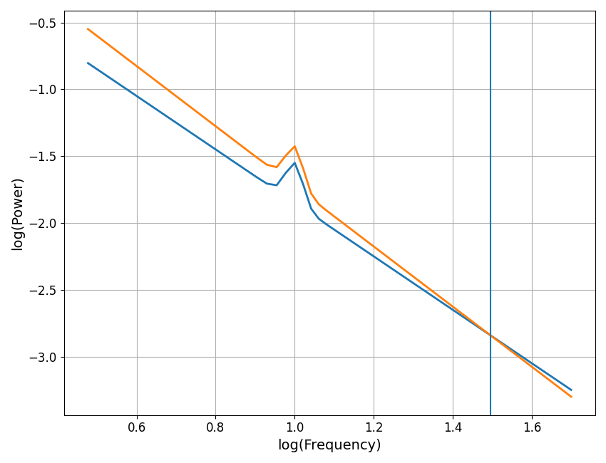
Rotate Different Amounts at Different Frequencies

Finally, let’s consider the case in which we rotate a spectrum by different delta exponents, and do so at different rotation frequencies.

As before, the changes in offset cancel out, and the total change in exponent is the difference of the two delta values.

However, in this case, the frequency of rotation between ‘B’ and ‘C’ is neither of the original rotation frequencies. To calculate the rotation frequency between ‘B’ and ‘C’, we can use the compute_rotation_frequency() function, which calculates the new relationship between ‘B’ and ‘C’, using the formula for how spectra are rotated.

# Settings for rotating power spectra
delta_exp_1 = 0.5
delta_exp_2 = 0.75
f_rotation_1 = 2
f_rotation_2 = 5

# Rotate a spectrum, different amounts, at different rotation frequencies
powers_1 = rotate_spectrum(freqs, powers, delta_exp_1, f_rotation_1)
powers_2 = rotate_spectrum(freqs, powers, delta_exp_2, f_rotation_2)

# Calculate the rotation frequency between the two spectra
f_rotation = compute_rotation_frequency(delta_exp_1, f_rotation_1,
                                        delta_exp_2, f_rotation_2)

# Print out the measured rotation frequency
template = "Rotation frequency: \t{:1.4f}"
print(template.format(f_rotation))

Rotation frequency:     31.2500

# Visualize the transformed power spectra, marking the rotation frequency
plot_spectra(freqs, [powers_1, powers_2],
             log_freqs=True, log_powers=True)
plt.axvline(np.log10(f_rotation))

<matplotlib.lines.Line2D object at 0x7f9627850250>