Exploring Data Components

This example explores the different data components, exploring the isolated aperiodic and periodic components as they are extracted from the data.

# Import FOOOF model objects
from fooof import FOOOF, FOOOFGroup

# Import function to plot power spectra
from fooof.plts.spectra import plot_spectra

# Import simulation functions to create some example data
from fooof.sim import gen_power_spectrum, gen_group_power_spectra

# Simulate example power spectrum
freqs, powers = gen_power_spectrum([1, 50], [0, 10, 1], [10, 0.25, 2], freq_res=0.25)

# Initialize model object and fit power spectrum
fm = FOOOF()
fm.fit(freqs, powers)

Data & Model Components

The model fit process includes procedures for isolating aperiodic and periodic components in the data, fitting each of these components separately, and then combining the model components as the final fit (see the Tutorials for further details on these procedures).

In doing this process, the model fit procedure computes and stores isolated data components, which are available in the model.

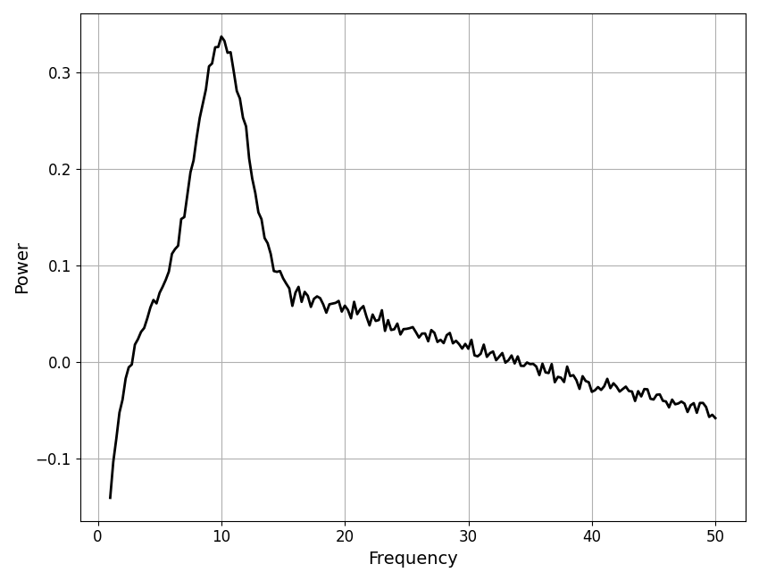
Full Data & Model Components

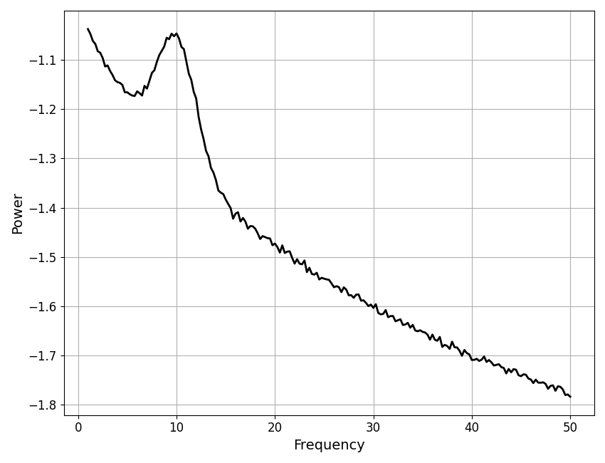
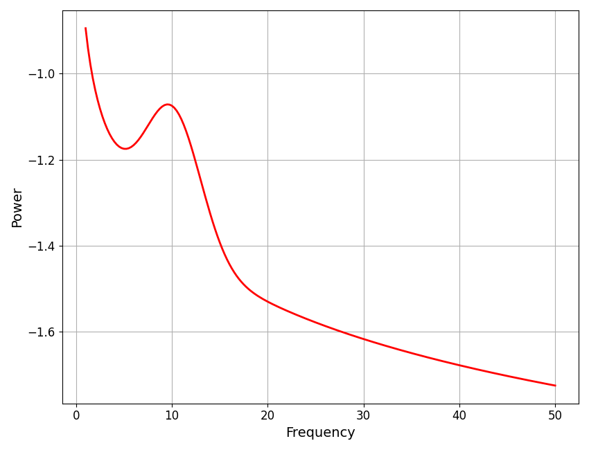
Before diving into the isolated data components, let’s check ‘full’ components, including the data (power_spectrum) and full model fit of a model object (fooofed_spectrum).

# Plot the original power spectrum data from the object
plot_spectra(fm.freqs, fm.power_spectrum, color='black')

# Plot the power spectrum model from the object
plot_spectra(fm.freqs, fm.fooofed_spectrum_, color='red')

Isolated Components

As well as the ‘full’ data & model components above, the model fitting procedure includes steps that result in isolated periodic and aperiodic components, in both the data and model. These isolated components are stored internally in the model.

To access these components, we can use the following getter methods:

• get_data(): allows for accessing data components

• get_model(): allows for accessing model components

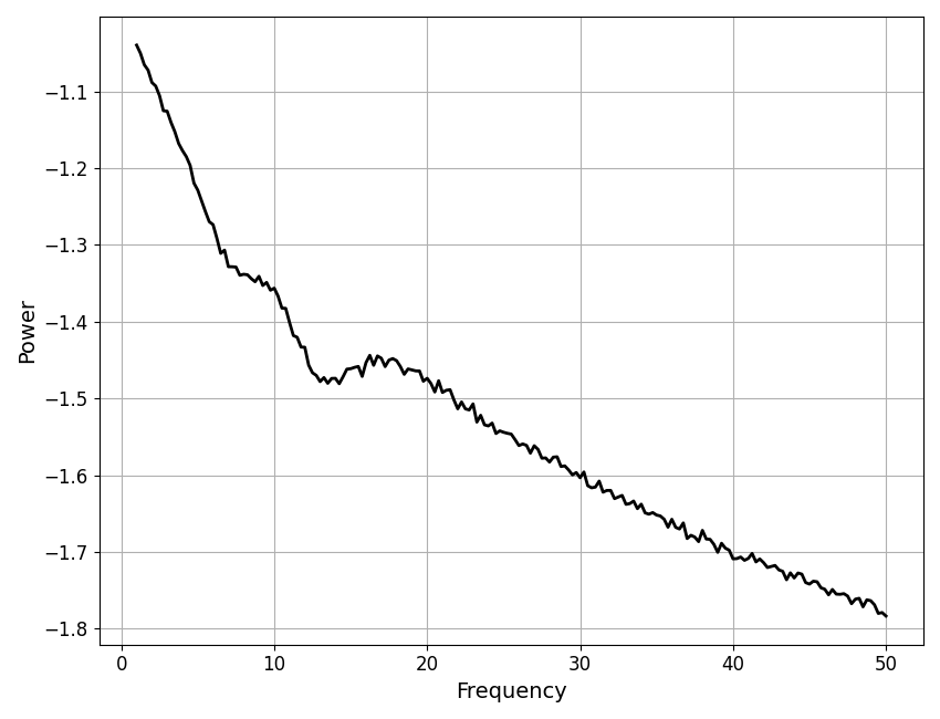
Aperiodic Component

To fit the aperiodic component, the model fit procedure includes a peak removal process.

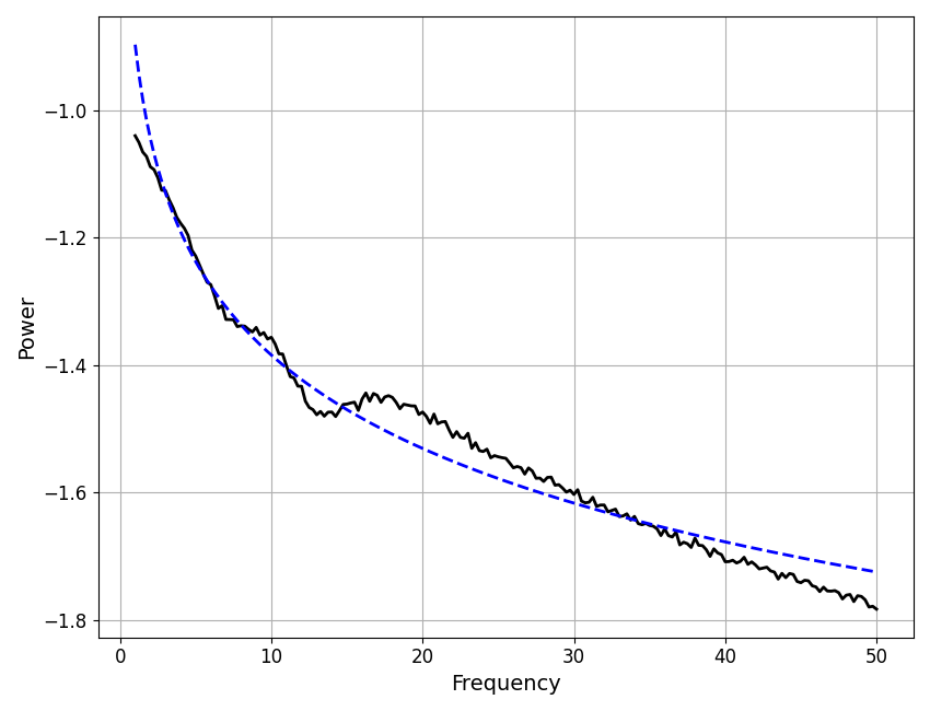
The resulting ‘peak-removed’ data component is stored in the model object, as well as the isolated aperiodic component model fit.

# Plot the peak removed spectrum data component
plot_spectra(fm.freqs, fm.get_data('aperiodic'), color='black')

# Plot the peak removed spectrum, with the model aperiodic fit
plot_spectra(fm.freqs, [fm.get_data('aperiodic'), fm.get_model('aperiodic')],
             colors=['black', 'blue'], linestyle=['-', '--'])

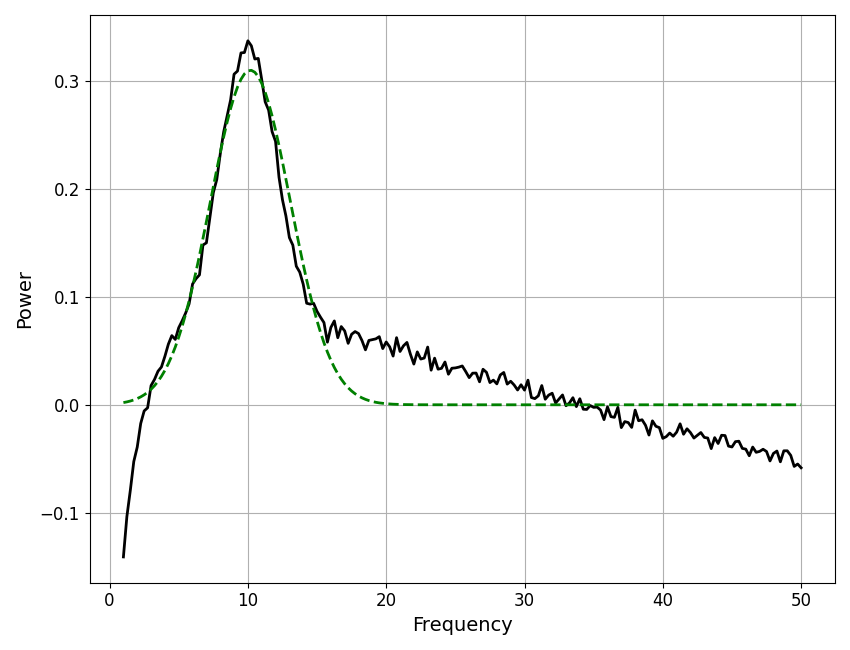
Periodic Component

To fit the periodic component, the model fit procedure removes the fit peaks from the power spectrum.

The resulting ‘flattened’ data component is stored in the model object, as well as the isolated periodic component model fit.

# Plot the flattened spectrum data component
plot_spectra(fm.freqs, fm.get_data('peak'), color='black')

# Plot the flattened spectrum data with the model peak fit
plot_spectra(fm.freqs, [fm.get_data('peak'), fm.get_model('peak')],
             colors=['black', 'green'], linestyle=['-', '--'])

Full Model Fit

The full model fit, which we explored earlier, is calculated as the combination of the aperiodic and peak fit, which we can check by plotting these combined components.

# Plot the full model fit, as the combination of the aperiodic and peak model components
plot_spectra(fm.freqs, [fm.get_model('aperiodic') + fm.get_model('peak')], color='red')

Linear vs Log Spacing

The above shows data components as they are available on the model object, and used in the fitting process - notable, in log10 spacing.

Some analyses may aim to use these isolated components to compute certain measures of interest on the data. However, when doing so, one may often want the linear power representations of these components.

Both the get_data and get_model methods accept a ‘space’ argument, whereby the user can specify whether the return the components in log10 or linear spacing.

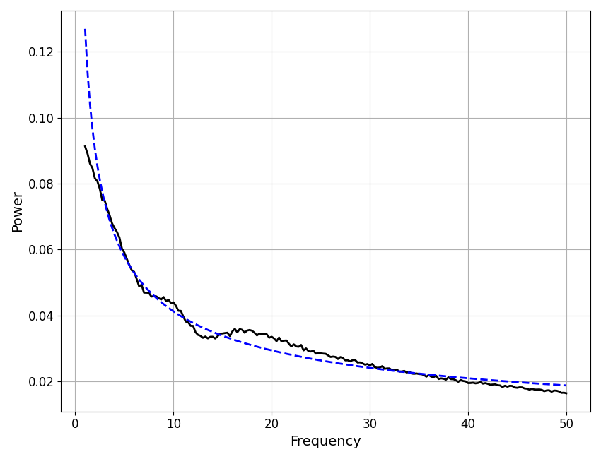
Aperiodic Components in Linear Space

First we can examine the aperiodic data & model components, in linear space.

# Plot the peak removed spectrum, with the model aperiodic fit
plot_spectra(fm.freqs, [fm.get_data('aperiodic', 'linear'), fm.get_model('aperiodic', 'linear')],
             colors=['black', 'blue'], linestyle=['-', '--'])

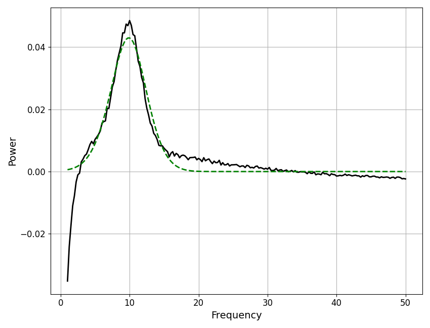
Peak Component in Linear Space

Next, we can examine the peak data & model components, in linear space.

# Plot the flattened spectrum data with the model peak fit
plot_spectra(fm.freqs, [fm.get_data('peak', 'linear'), fm.get_model('peak', 'linear')],
             colors=['black', 'green'], linestyle=['-', '--'])

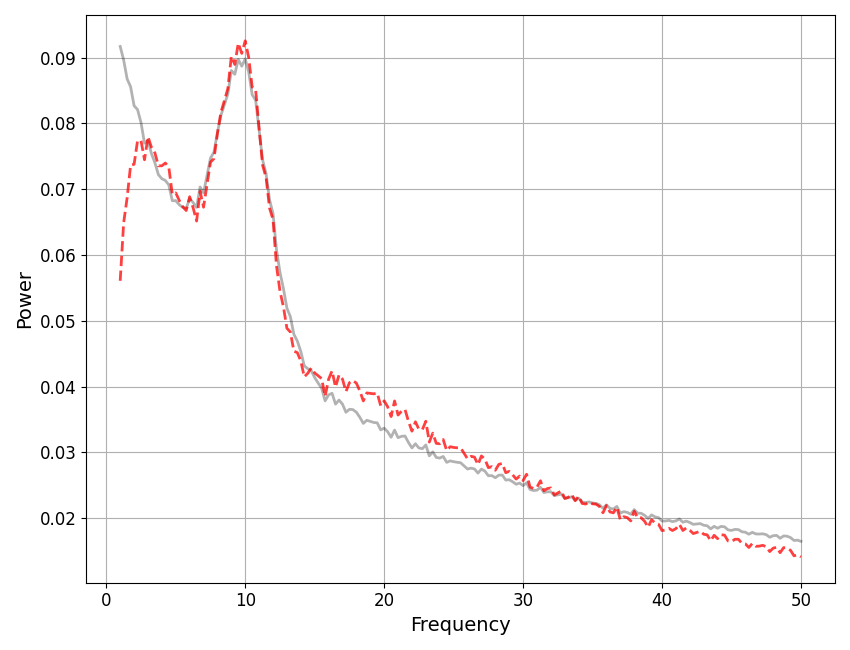
Linear Space Additive Model

Note that specifying ‘linear’ does not simply unlog the data components to return them in linear space, but instead defines the space of the additive data definition such that power_spectrum = aperiodic_component + peak_component (for data and/or model).

We can see this by plotting the linear space data (or model) with the corresponding aperiodic and periodic components summed together. Note that if you simply unlog the components and sum them, they does not add up to reflecting the full data / model.

# Plot the linear data, showing the combination of peak + aperiodic matches the full data
plot_spectra(fm.freqs,
             [fm.get_data('full', 'linear'),
              fm.get_data('aperiodic', 'linear') + fm.get_data('peak', 'linear')],
             linestyle=['-', 'dashed'], colors=['black', 'red'], alpha=[0.3, 0.75])

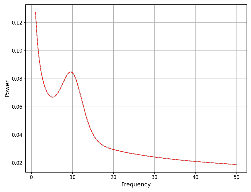
# Plot the linear model, showing the combination of peak + aperiodic matches the full model
plot_spectra(fm.freqs,
             [fm.get_model('full', 'linear'),
              fm.get_model('aperiodic', 'linear') + fm.get_model('peak', 'linear')],
             linestyle=['-', 'dashed'], colors=['black', 'red'], alpha=[0.3, 0.75])

Notes on Analyzing Data & Model Components

The functionality here allows for accessing the model components in log space (as used by the model for fitting), as well as recomputing in linear space.

If you are aiming to analyze these components, it is important to consider which version of the data you should analyze for the question at hand, as there are key differences to the different representations. Users who wish to do so post-hoc analyses of these data and model components should consider the benefits and limitations the different representations.