Conflating Periodic & Aperiodic Changes

Demonstrating how changes in periodic & aperiodic parameters can be conflated.

This example is a code implementation and quantitatively exact version of Figure 1 from the Parameterizing Neural Power Spectra paper.

Measuring Neural Activity

In electrophysiological data analysis, we often wish to measure and interpret changes in particular aspects of our data, for example, measuring changes in the power of a frequency band of interest.

In this example, we will examine how using predefined frequency ranges to measure and then interpret differences from power spectra can lead to misinterpretations in the face of complex data in which multiple different aspects of the data can change or vary within and between recordings.

We conceptualize neural data as complex data that contains multiple ‘components’, which we categorize as periodic and aperiodic, and note that each of these components can also have multiple parameters, each of which could vary.

To briefly recap, these components and parameters include:

• aperiodic activity, the 1/f-like aspect of the data, described, at minimum with:

  • exponent

  • offset

• periodic activity, peaks in the power spectrum, each with a:

  • center frequency

  • power

  • bandwidth

# Import numpy & matplotlib
import numpy as np
import matplotlib.pyplot as plt

# Import simulation, utility, and plotting tools
from fooof.bands import Bands
from fooof.utils import trim_spectrum
from fooof.sim.gen import gen_power_spectrum
from fooof.plts.spectra import plot_spectra_shading

# Settings for plotting
log_freqs = True
log_powers = True
shade_color = '#0365C0'

Simulating Data

For this example, we will use simulated data, and consider the example case of investigating differences in alpha activity.

We will start by simulating a baseline power spectrum, with an alpha peak, and concurrent aperiodic activity. We will also simulate several altered versions of this spectrum, each which a change in a specific parameter of the power spectrum.

# Define our bands of interest
bands = Bands({'alpha' : (8, 12)})

# Simulation Settings
nlv = 0
f_res = 0.1
f_range = [3, 35]

# Define baseline parameter values
ap_base = [0, 1.5]
pe_base = [[10, 0.5, 1], [22, 0.2, 2]]

# Define parameters sets with changes in each parameter
pw_diff = [[10, 0.311, 1], [22, 0.2, 2]]
cf_diff = [[11.75, 0.5, 1], [22, 0.2, 2]]
off_diff = [-0.126, 1.5]
exp_diff = [-0.87, 0.75]

# Create baseline power spectrum, to compare to
freqs, powers_base = gen_power_spectrum(f_range, ap_base, pe_base, nlv, f_res)

# Create comparison power spectra, with differences in different parameters of the data
_, powers_pw = gen_power_spectrum(f_range, ap_base, pw_diff, nlv, f_res)
_, powers_cf = gen_power_spectrum(f_range, ap_base, cf_diff, nlv, f_res)
_, powers_off = gen_power_spectrum(f_range, off_diff, pe_base, nlv, f_res)
_, powers_exp = gen_power_spectrum(f_range, exp_diff, pe_base, nlv, f_res)

# Collect the comparison power spectra together
all_powers = {
    'Alpha Power Change' : powers_pw,
    'Alpha Frequency Change' : powers_cf,
    'Offset Change' : powers_off,
    'Exponent Change' : powers_exp
}

Plotting Power Spectra

Now that we have our power spectra simulated, let’s plot them all together.

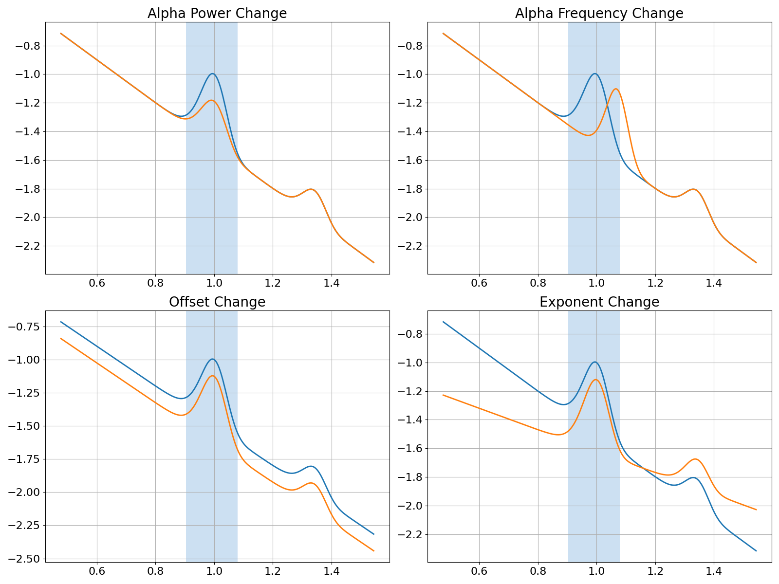
In the visualization below, we can see that we have created four sets of comparisons, where each has a change in one parameter of the data.

Specifically, these changes are:

• a change in alpha power, part of the periodic component

• a change in alpha center frequency, part of the periodic component

• a change in the offset of the aperiodic component

• a change in the exponent of the aperiodic component

# Plot and compare all of our power spectra
fig, axes = plt.subplots(2, 2, figsize=(16, 12))
for ax, (title, powers) in zip(axes.reshape(-1), all_powers.items()):

    # Create spectrum plot, with alpha band of interest shaded in
    plot_spectra_shading(freqs, [powers_base, powers],
                         bands.alpha, shade_colors=shade_color,
                         log_freqs=log_freqs, log_powers=log_powers, ax=ax)

    # Add the title, and do some plot styling
    ax.set_title(title, {'fontsize' : 20})
    ax.xaxis.label.set_visible(False)
    ax.yaxis.label.set_visible(False)

Comparing Power Spectra

Now let’s compare our different power spectra, in terms of band-specific power measures.

To do so, we will first define a helper function that calculates the average power in a band.

Then, for each pair, consisting of the baseline power spectrum and an adapted version in which one parameter has been changed, we can measure the change in band specific activity relating to this change.

def calc_avg_power(freqs, powers, freq_range):
    """Helper function to calculate average power in a band."""

    _, band_powers = trim_spectrum(freqs, powers, freq_range)
    avg_power = np.mean(band_powers)

    return avg_power

# Calculate the amount of alpha power in the baseline power spectrum
base_alpha = calc_avg_power(freqs, powers_base, bands.alpha)

# Calculate the different in alpha power for each of our comparison pairs
for title, powers in all_powers.items():
    print('{:20s}\t {:1.4f}'.format(\
        title, calc_avg_power(freqs, powers, bands.alpha) - base_alpha))

Alpha Power Change       -0.0171
Alpha Frequency Change   -0.0171
Offset Change            -0.0171
Exponent Change          -0.0171

We can see that all of these cases have the exact measured change in alpha power!

However, given that we know exactly what was changed in the simulated data, we know that a change in alpha power is only the correct interpretation in one of the cases that we simulated.

For all the other comparisons, the change in the data is not a change in band specific power. Despite this, the common analysis approach measures it as such.

This shows how measurements that are supposed to reflect band specific power changes can easily be conflated and misinterpreted, as they can be driven by other changes in the data.

Spectra Without any Oscillations

So far we have considered the case in which the goal is to analyze and measure alpha power activity, in a scenario in which there actually is alpha activity.

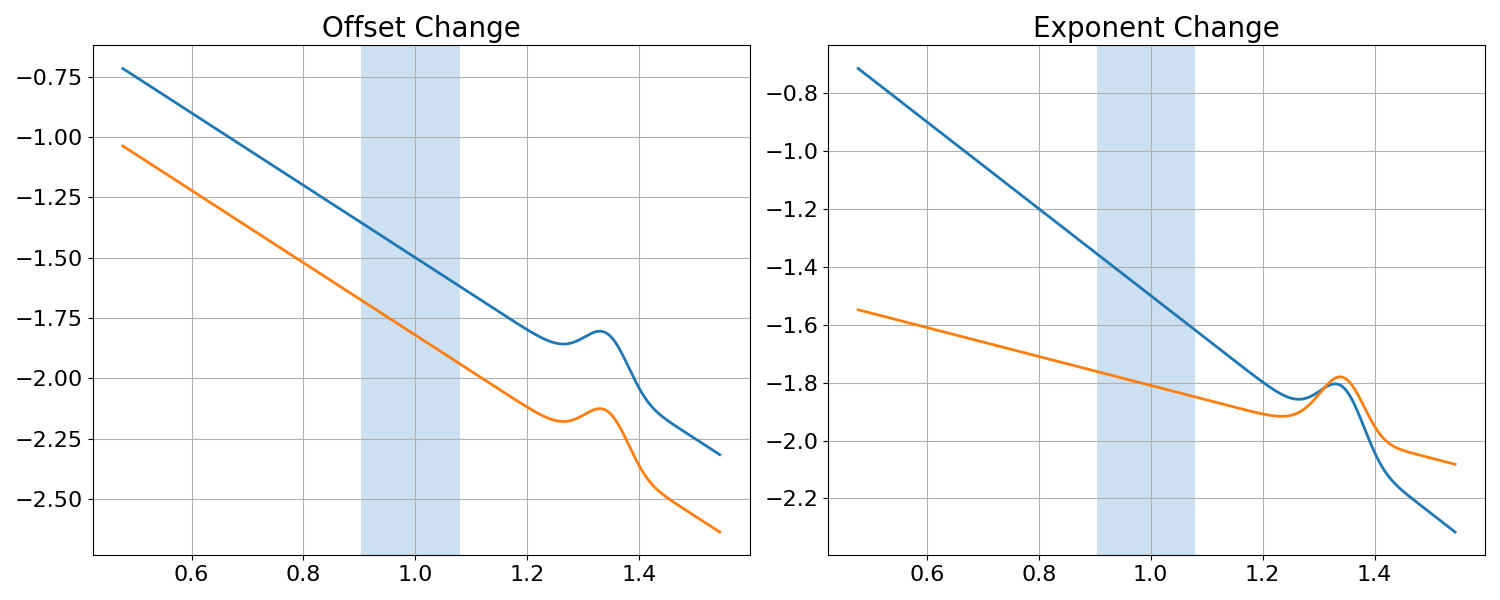
However, we can also consider the possible scenario of analyzing alpha power (or, by analogy, any other band), in cases in which there is no band-specific power.

To do so, we will simulate, plot and measure a new set of data, with the same set up as above, but without adding any alpha peaks to the spectra.

# Redefine baseline with no alpha
pe_base_na = [[22, 0.2, 2]]

# Redefine changes in for each parameter
off_diff_na = [-0.321, 1.5]
exp_diff_na = [-1.31, 0.5]

# Create baseline power spectrum, to compare to
freqs, powers_noa_base = gen_power_spectrum(f_range, ap_base, pe_base_na, nlv, f_res)

# Collect all powers together,
all_powers_na = {'Offset Change' : \
                    gen_power_spectrum(f_range, off_diff_na, pe_base_na, nlv, f_res)[1],
                 'Exponent Change' : \
                    gen_power_spectrum(f_range, exp_diff_na, pe_base_na, nlv, f_res)[1]}

# Plot and compare spectra with no alpha
fig, axes = plt.subplots(1, 2, figsize=(15, 6))
for ax, (title, powers) in zip(axes.reshape(-1), all_powers_na.items()):

    # Create spectrum plot, with alpha band of interest shaded in
    plot_spectra_shading(freqs, [powers_noa_base, powers],
                         bands.alpha, shade_colors=shade_color,
                         log_freqs=log_freqs, log_powers=log_powers, ax=ax)

    # Add the title, and do some plot styling
    ax.set_title(title, {'fontsize' : 20})
    ax.xaxis.label.set_visible(False)
    ax.yaxis.label.set_visible(False)

# Calculate and compare the difference of 'alpha' power
base_noa_power = calc_avg_power(freqs, powers_noa_base, [8, 12])
for title, powers in all_powers_na.items():
    print('{:20s}\t {:1.4f}'.format(\
        title, calc_avg_power(freqs, powers, [8, 12]) - base_noa_power))

Offset Change            -0.0171
Exponent Change          -0.0171

In the plots and analyses above, we can see that when analyzing a predefined narrow-band frequency range, we can get the same measured difference in ‘alpha’ power between spectra, even if there is no evidence of an oscillation at all.

Conclusion

In the simulations above, we have shown that changes in multiple different parameters can lead to the same measured difference in band-specific power.

In any given case in which narrow-band ranges are used, any of these changes, or a combination of them, could be contributing to the measured changes.

As an alternative to analyzing narrow-band power, parameterizing power spectra offers an approach that can measure which parameters of the data are changing, and in what ways.