Band Ratio Measures

Exploring how band ratio measures relate to periodic & aperiodic activity.

Introduction

Band ratios measures are a relatively common measure, proposed to measure oscillatory, or periodic, activity.

They are typically calculated as:

\[BR = \frac{avg(low band power)}{avg(high band power)}\]

In this notebook we will explore this measure in the context of conceptualizing neural power spectra as a combination of aperiodic and periodic activity.

Band Ratios Project

This example offers a relatively quick demonstration of how band ratios measures relate to periodic and aperiodic activity.

We have completed a full project investigating methodological properties of band ratio measures, which is available here.

# Import numpy and matplotlib
import numpy as np
import matplotlib.pyplot as plt

# Import simulation, utility, and plotting tools
from fooof.bands import Bands
from fooof.utils import trim_spectrum
from fooof.sim.gen import gen_power_spectrum
from fooof.sim.utils import set_random_seed
from fooof.plts.spectra import plot_spectra_shading

# General Settings

# Define band definitions
bands = Bands({'theta' : [4, 8], 'beta' : [20, 30]})

# Define helper variables for indexing peak data
icf, ipw, ibw = 0, 1, 2

# Plot settings
shade_color = '#0365C0'

Simulating Data

For this example, we will use simulated data. Let’s start by simulating a a baseline power spectrum.

# Simulation Settings
nlv = 0
f_res = 0.1
f_range = [1, 35]

# Define default aperiodic values
ap = [0, 1]

# Define default periodic values for band specific peaks
theta = [6, 0.4, 1]
alpha = [10, 0.5, 0.75]
beta  = [25, 0.3, 1.5]

# Set random seed, for consistency generating simulated data
set_random_seed(21)

# Simulate a power spectrum
freqs, powers = gen_power_spectrum(f_range, ap, [theta, alpha, beta], nlv, f_res)

Calculating Band Ratios

Band ratio measures are a ratio of power between defined frequency bands.

We can now define a function we can use to calculate band ratio measures, and apply it to our baseline power spectrum.

For this example, we will be using the theta / beta ratio, which is the most commonly applied band ratio measure.

Note that it doesn’t matter exactly which ratio measure or which frequency band definitions we use, as the general properties demonstrated here generalize to different bands and ranges.

def calc_band_ratio(freqs, powers, low_band, high_band):
    """Helper function to calculate band ratio measures."""

    # Extract frequencies within each specified band
    _, low_band = trim_spectrum(freqs, powers, low_band)
    _, high_band = trim_spectrum(freqs, powers, high_band)

    # Calculate average power within each band, and then the ratio between them
    ratio = np.mean(low_band) / np.mean(high_band)

    return ratio

# Plot the power spectrum, shading the frequency bands used for the ratio
plot_spectra_shading(freqs, powers, [bands.theta, bands.beta],
                     color='black', shade_colors=shade_color,
                     log_powers=True, linewidth=3.5)

# Calculate a band ratio measure
tbr = calc_band_ratio(freqs, powers, bands.theta, bands.beta)
print('Calculate theta / beta ratio is :\t {:1.2f}'.format(tbr))

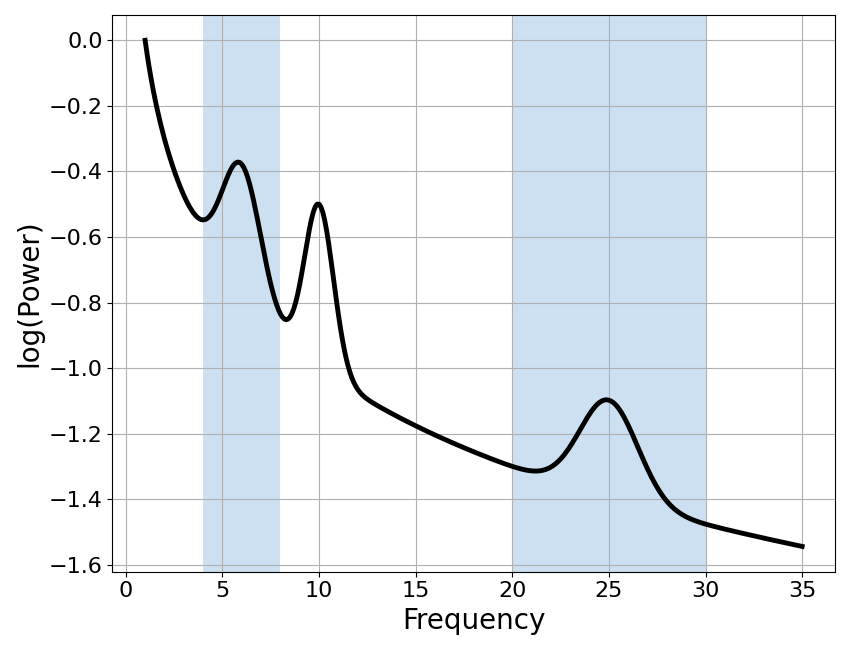
Calculate theta / beta ratio is :        5.74

Periodic Impacts on Band Ratio Measures

Typical investigations involving band ratios compare differences in band ratio measures within and between subjects. The typical interpretation of band ratio measures is that they relate to the relative power between two bands.

Next, lets simulate data that varies across different periodic parameters of the data, and see how this changes our measured theta / beta ratio, as compared to our baseline power spectrum.

# Define a helper function for updating parameters
from copy import deepcopy
def upd(data, index, value):
    """Return a updated copy of an array."""
    out = deepcopy(data)
    out[index] = value
    return out

# Simulate and collect power spectra with changes in each periodic parameter
spectra = {
    'Theta Frequency' : None,
    'Theta Power' : gen_power_spectrum(\
        f_range, ap, [upd(theta, ipw, 0.5041), alpha, beta], nlv, f_res)[1],
    'Theta Bandwidth' : gen_power_spectrum(\
        f_range, ap, [upd(theta, ibw, 1.61), alpha, beta], nlv, f_res)[1],
    'Alpha Frequency' : gen_power_spectrum(\
        f_range, ap, [theta, upd(alpha, icf, 8.212), beta], nlv, f_res)[1],
    'Alpha Power' : None,
    'Alpha Bandwidth' : gen_power_spectrum(\
        f_range, ap, [theta, upd(alpha, ibw, 1.8845), beta], nlv, f_res)[1],
    'Beta Frequency' : gen_power_spectrum(\
        f_range, ap, [theta, alpha, upd(beta, icf, 19.388)], nlv, f_res)[1],
    'Beta Power' : gen_power_spectrum(\
        f_range, ap, [theta, alpha, upd(beta, ipw, 0.1403)], nlv, f_res)[1],
    'Beta Bandwidth' : gen_power_spectrum(\
        f_range, ap, [theta, alpha, upd(beta, ibw, 0.609)], nlv, f_res)[1],
}

# Calculate changes in theta / beta ratios
for label, spectrum in spectra.items():
    if spectrum is not None:
        print('TBR difference from   {:20}   is \t {:1.3f}'.format(\
            label, tbr - calc_band_ratio(freqs, spectrum, bands.theta, bands.beta)))

TBR difference from   Theta Power            is          -1.000
TBR difference from   Theta Bandwidth        is          -1.000
TBR difference from   Alpha Frequency        is          -1.000
TBR difference from   Alpha Bandwidth        is          -1.000
TBR difference from   Beta Frequency         is          -1.000
TBR difference from   Beta Power             is          -1.000
TBR difference from   Beta Bandwidth         is          -1.000

# Create figure of periodic changes
title_settings = {'fontsize': 16, 'fontweight': 'bold'}
fig, axes = plt.subplots(3, 3, figsize=(15, 14))

for ax, (label, spectrum) in zip(axes.flatten(), spectra.items()):

    if spectrum is None: continue

    plot_spectra_shading(freqs, [powers, spectrum],
                         [bands.theta, bands.beta], shade_colors=shade_color,
                         log_freqs=False, log_powers=True, ax=ax)

    ax.set_title(label, **title_settings)
    ax.set_xlim([0, 35]); ax.set_ylim([-1.75, 0])
    ax.xaxis.label.set_visible(False)
    ax.yaxis.label.set_visible(False)

# Turn off empty axes & space out axes
fig.subplots_adjust(hspace=.3, wspace=.3)
_ = [ax.axis('off') for ax in [axes[0, 0], axes[1, 1]]]

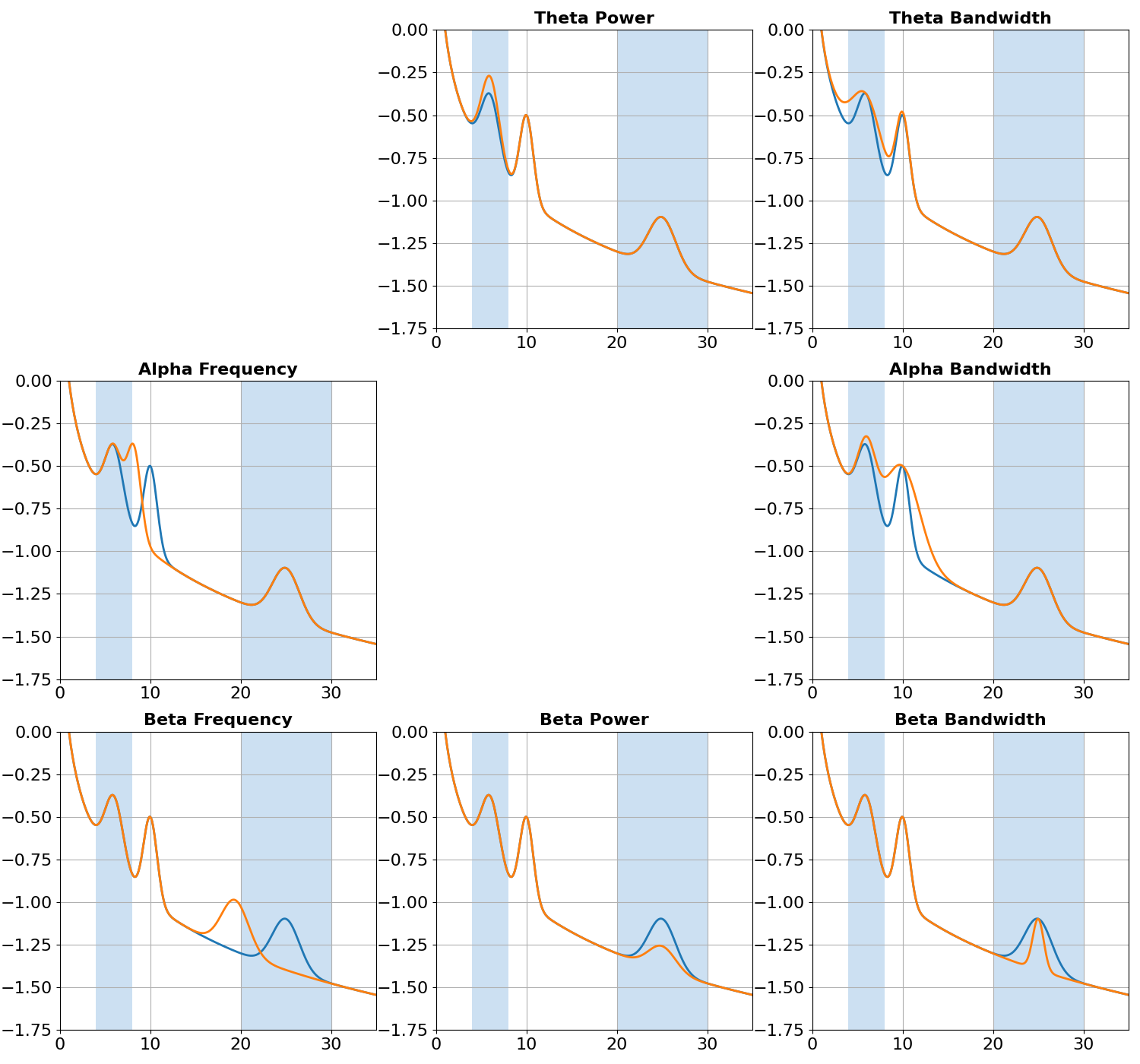
In the simulations above, we systematically manipulated each parameter of each of the three different band peaks present in our data. For 7 of the 9 possible changes, we can do so in a way that creates an identical change in the measured band ratio measure.

Band ratio measures are therefore not specific to band power differences, but rather can reflect multiple different changes across multiple different periodic parameters.

Aperiodic Impacts on Band Ratio Measures

Next, we can also examine if changes in aperiodic properties of the data can also impact band ratio measures. We will explore changes in the aperiodic exponent, with and without overlying peaks.

To do so, we will use the same approach to simulating, comparing, and plotting data as above (though note that the code to do so has been condensed in the next section).

# Simulate and collect power spectra with changes in aperiodic parameters
exp_spectra = {
    'Exponent w Peaks' : \
        [powers,
         gen_power_spectrum(f_range, [0.13, 1.1099],
                            [theta, alpha, beta], nlv, f_res)[1]],
    'Exponent w/out Peaks' : \
        [gen_power_spectrum(f_range, ap, [], nlv, f_res)[1],
         gen_power_spectrum(f_range, [0.13, 1.1417], [], nlv, f_res)[1]]}

# Calculate & plot changes in theta / beta ratios
fig, axes = plt.subplots(1, 2, figsize=(15, 6))
fig.subplots_adjust(wspace=.3)
for ax, (label, (comparison, spectrum)) in zip(axes, exp_spectra.items()):
    print('\tTBR difference from   {:20}   is \t {:1.3f}'.format(label, \
        calc_band_ratio(freqs, comparison, bands.theta, bands.beta) - \
        calc_band_ratio(freqs, spectrum, bands.theta, bands.beta)))
    plot_spectra_shading(freqs, [comparison, spectrum],
                         [bands.theta, bands.beta],
                         shade_colors=shade_color,
                         log_freqs=False, log_powers=True, ax=ax)
    ax.set_title(label, **title_settings)
    ax.set_xlim([0, 35]); ax.set_ylim([-1.75, 0])

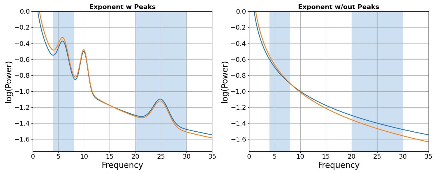
TBR difference from   Exponent w Peaks       is          -1.000
TBR difference from   Exponent w/out Peaks   is          -1.000

In these simulations, we again see that we can obtain the same measured difference in band ratio measures from differences in the aperiodic properties of the data. This is true even if there are no periodic peaks present at all.

This shows that band ratio measures are not even specific to periodic activity, and can be driven by changes in aperiodic activity.

Conclusion

Band ratio measures are supposed to reflect the relative power of rhythmic neural activity.

However, here we can see that band ratio measures are actually under-determined in that many different changes of both periodic and aperiodic parameters can affect band ratio measurements - including aperiodic changes when there is no periodic activity.

For this reason, we conclude that band-ratio measures, by themselves, are an insufficient measure of neural activity. We propose that approaches such as parameterizing power spectra are more specific for adjudicating what is changing in neural data.

For more investigation into band ratios, their methodological issues, applications to real data, and a comparison to parameterizing power spectra, see the full project here,