Note
Go to the end to download the full example code.
‘Oscillations’ as Peaks
Exploring the idea of oscillations as peaks of power.
# Imports from NeuroDSP to simulate & plot time series
from neurodsp.sim import sim_powerlaw, sim_oscillation, sim_combined, set_random_seed
from neurodsp.spectral import compute_spectrum
from neurodsp.plts import plot_time_series, plot_power_spectra
from neurodsp.utils import create_times
# Define simulation settings
n_seconds = 30
fs = 1000

# Create a times vector
times = create_times(n_seconds, fs)
Frequency Specific Power
Part of the motivation behind spectral parameterization is dissociating aperiodic activity, with no characteristic frequency, to periodic power, which is defined as having frequency specific power. This leads to the idea of oscillations as ‘peaks’ of power in the power spectrum, which can be detected and measured.
In this exploration, we will use simulated time series to examine how rhythmic signals do display as ‘peaks’ of power in frequency domain representations. We will also explore some limitations of this idea.
# Simulate an ongoing sine wave
sine_wave = sim_oscillation(n_seconds, fs, 10)

# Visualize the sine wave
plot_time_series(times, sine_wave, xlim=[0, 5])
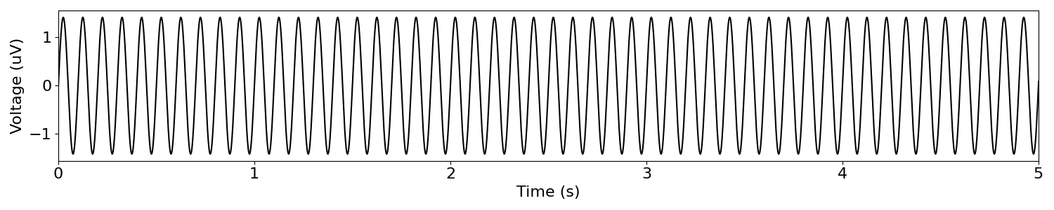
In the above, we simulated a pure sinusoid, at 10 Hz.
# Compute the power spectrum of the sine wave
freqs, powers = compute_spectrum(sine_wave, fs)

# Visualize the power spectrum
plot_power_spectra(freqs, powers)
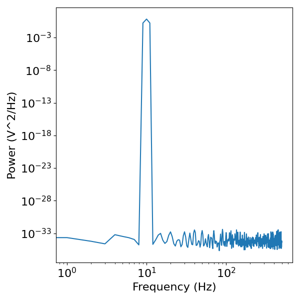
The power spectrum of the sine wave shows a clear peak of power at 10 Hz, reflecting the simulated rhythm, with close to zero power at all other frequencies.
This is characteristic of a sine wave, and demonstrates the basic idea of considering oscillations as peaks of power in the power spectrum.
Next lets examine a more complicated signal, with multiple components.
# Define components for a combined signal
components = {
    'sim_oscillation' : {'freq' : 10},
    'sim_powerlaw' : {'exponent' : -1},
}

# Simulate a combined signal
sig = sim_combined(n_seconds, fs, components)

# Visualize the time series
plot_time_series(times, sig, xlim=[0, 5])
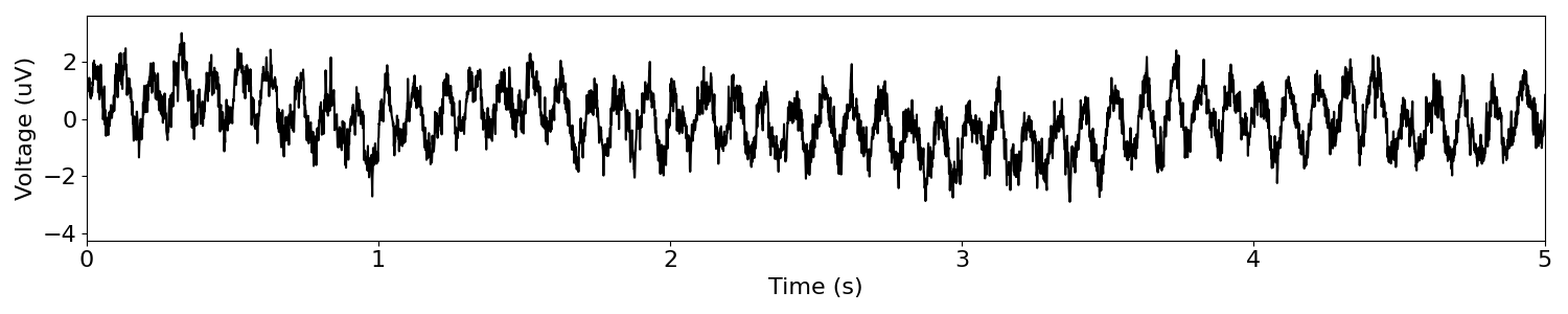
Here we see a simply simulation meant to be closer to neural data, reflecting an oscillatory component, as well as an aperiodic component, which contributes power across all frequencies.
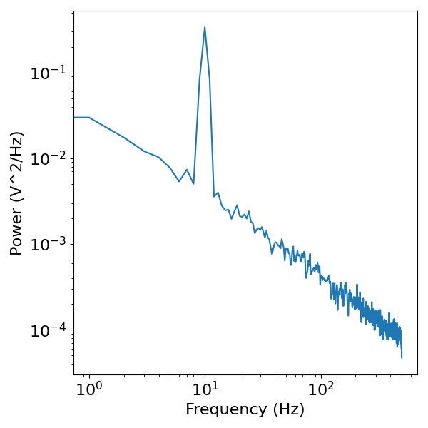
# Compute the power spectrum of the sine wave
freqs, powers = compute_spectrum(sig, fs)

# Visualize the power spectrum
plot_power_spectra(freqs, powers)
Interim Conclusion
In the power spectrum of the combined signal, we can still the peak of power at 10 Hz, as well as the pattern of power across all frequencies contributed by the aperiodic component.
This basic example serves as the basic motivation for spectral parameterization. In this simulated example, we know there are two components, and so a procedure for detecting the peaks and measuring the pattern of aperiodic power (as is done in spectral parameterization) provides a method to measuring these components in the data.
Harmonic Peaks
The above seeks to demonstrate the basic idea whereby a peak of power _may_ reflect an oscillation at that frequency, where as patterns of power across all frequencies likely reflect aperiodic activity.
In the this section, we will further explore peaks of power in the frequency domain, showing that not every peak necessarily reflect an independent oscillation.
To do so, we will start by simulating a non-sinusoidal oscillation.
# Simulate a sawtooth wave
sawtooth = sim_oscillation(n_seconds, fs, 10, 'sawtooth', width=0.5)

# Visualize the sine wave
plot_time_series(times, sawtooth, xlim=[0, 5])
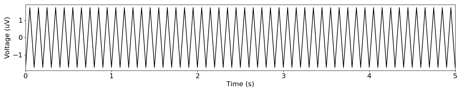
In the above, we can see that there is again an oscillation, although it is not sinusoidal.
# Compute the power spectrum of the sine wave
freqs, powers = compute_spectrum(sawtooth, fs)

# Visualize the power spectrum
plot_power_spectra(freqs, powers)
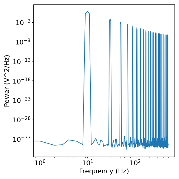
Note the 10 Hz peak, as well as the additional peaks in the frequency domain.
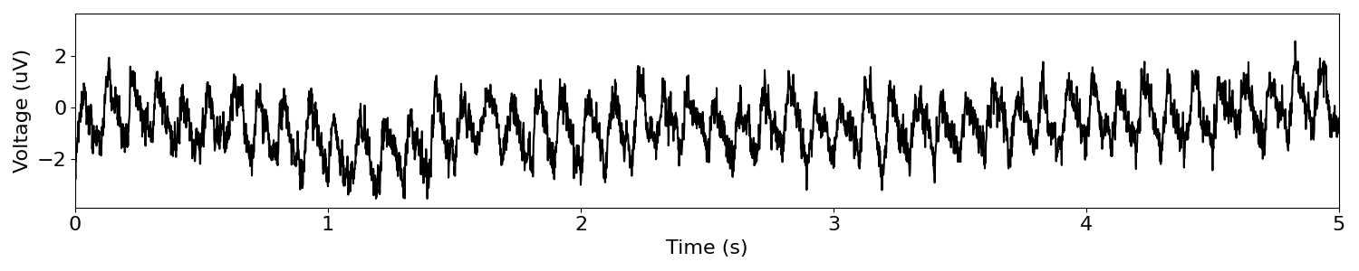
Before further discussing this, let’s create an example with an aperiodic component.
# Define components for a combined signal
components = {
    'sim_oscillation' : {'freq' : 10, 'cycle' : 'sawtooth', 'width' : 0.25},
    'sim_powerlaw' : {'exponent' : -1.},
}

# Simulate a combined signal
sig = sim_combined(n_seconds, fs, components)

# Visualize the time series
plot_time_series(times, sig, xlim=[0, 5])
# Compute the power spectrum of the sine wave
freqs, powers = compute_spectrum(sig, fs)

# Visualize the power spectrum
plot_power_spectra(freqs, powers)
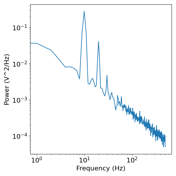
In the power spectrum above, we see that there is a peak of power at the fundamental frequency of the rhythm (10 Hz), but there are also numerous other peaks. These additional peaks are ‘harmonics’, and that are components of the frequency domain representation that reflect the non-sinusoidality of the time domain signal.
This serves as the basic motivation for the claim that although a peak _may_ reflect an independent oscillation, this need not be the case, as a given peak could simply be the harmonic of an asymmetric oscillation at a different frequency. For this reason, the number of peaks in a model can not be interpreted as the number of oscillations in a signal.
Total running time of the script: (0 minutes 1.690 seconds)