Finding ‘Oscillations’ With Filters

Examining the results of filtering aperiodic signals.

Filtering Signals

A common component of many analyses of neural time series is to apply filters, typically to try to extract information from frequency bands of interest.

However, one thing to keep in mind is that signals with aperiodic activity will always contain power at all frequencies. One of the corollaries of thinking of neural signals as containing aperiodic activity, is that there is always power within any arbitrarily defined frequency range. This power does not necessarily entail any periodic activity, but it can look like periodic activity when applying transforms such as narrow-band filters.

In this notebook we will simulate purely aperiodic signals, and apply filters to them, to explore these ideas.

# Import numpy and matplotlib
import numpy as np
import matplotlib.pyplot as plt

# Import the Bands object, for managing frequency band definitions
from fooof.bands import Bands

# Imports from NeuroDSP to simulate & plot time series
from neurodsp.sim import sim_powerlaw, set_random_seed
from neurodsp.filt import filter_signal
from neurodsp.plts import plot_time_series
from neurodsp.utils import create_times

# Define our bands of interest
bands = Bands({'delta' : [2, 4],
               'theta' : [4, 8],
               'alpha' : [8, 13],
               'beta' : [13, 30],
               'low_gamma' : [30, 50],
               'high_gamma' : [50, 150]})

Simulating Data

We will use simulated data for this example, to create some example aperiodic signals, that we can then apply filters to. First, let’s simulate some data.

# Simulation settings
s_rate = 1000
n_seconds = 4
times = create_times(n_seconds, s_rate)

# Set random seed, for consistency generating simulated data
set_random_seed(21)

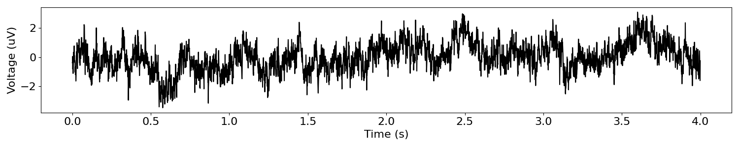
# Simulate a signal of aperiodic activity: pink noise
sig = sim_powerlaw(n_seconds, s_rate, exponent=-1)

# Plot our simulated time series
plot_time_series(times, sig)

Filtering Aperiodic Signals

Now that we have a simulated signal, let’s filter it into each of our frequency bands.

To do so, we will loop across our band definitions, and plot the filtered version of the signal.

# Apply band-by-band filtering of our signal into each defined frequency band
_, axes = plt.subplots(len(bands), 1, figsize=(12, 15))
for ax, (label, f_range) in zip(axes, bands):

    # Filter the signal to the current band definition
    band_sig = filter_signal(sig, s_rate, 'bandpass', f_range)

    # Plot the time series of the current band, and adjust plot aesthetics
    plot_time_series(times, band_sig, title=label + ' ' + str(f_range), ax=ax,
                     xlim=(0, n_seconds), ylim=(-1, 1), xlabel='')

/Users/tom/opt/anaconda3/lib/python3.8/site-packages/neurodsp/plts/style.py:101: UserWarning: The figure layout has changed to tight
  plt.tight_layout()

As we can see, filtering a signal with aperiodic activity into arbitrary frequency ranges returns filtered signals that look like rhythmic activity.

Also, because our simulated signal has some random variation, the filtered components also exhibit some fluctuations.

Overall, we can see from filtering this signal that:

• narrow band filters return rhythmic looking outputs

• filtering a signal with aperiodic activity will always return non-zero outputs

• there can be dynamics in the filtered results, due to variations of the aperiodic properties of the input signal

In this case, recall that our simulated signal contains no periodic activity. Altogether, this can be taken as example that just because time series can be represented as and decomposed into sinusoids, this does not indicate that these signals, or resulting decompositions, reflect rhythmic activity.

Observing Changes in Filtered Signals

Next, let’s consider what it looks like if you filter a signal that contains changes in the aperiodic activity.

For this example, we will simulate a signal, with an abrupt change in the aperiodic activity.

We will then filter this signal into narrow-band frequency ranges, to observe how changes in aperiodic activity appear in filtered data.

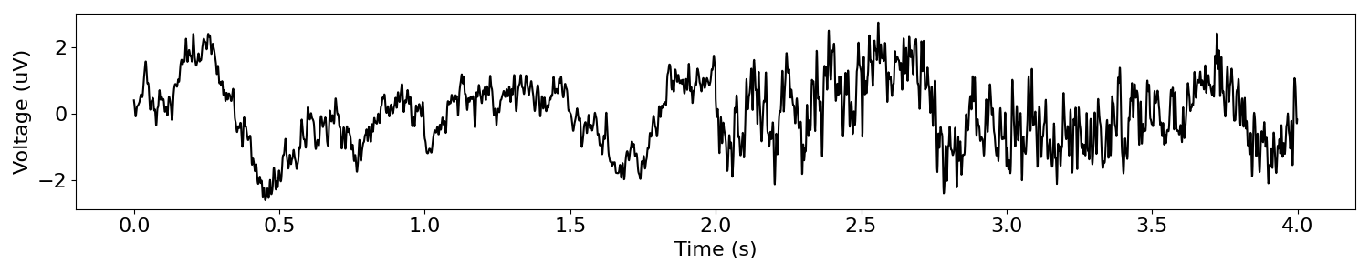
# Simulate a two signals with different aperiodic activity
sig_comp1 = sim_powerlaw(n_seconds/2, s_rate, exponent=-1.5, f_range=(None, 150))
sig_comp2 = sim_powerlaw(n_seconds/2, s_rate, exponent=-1, f_range=(None, 150))

# Combine each component signal to create a signal with a shift in aperiodic activity
sig_delta_ap = np.hstack([sig_comp1, sig_comp2])

# Plot our time series, with a shift in aperiodic activity
plot_time_series(times, sig_delta_ap)

Let’s first filter this signal in a low-frequency range that is typically examined for oscillatory activity, using the beta band as an example.

# Filter the signal to the current band definition
band_sig = filter_signal(sig_delta_ap, s_rate, 'bandpass', bands.beta)

# Plot the filtered time series
plot_time_series(times, band_sig, xlim=(0, n_seconds), ylim=(-1, 1))

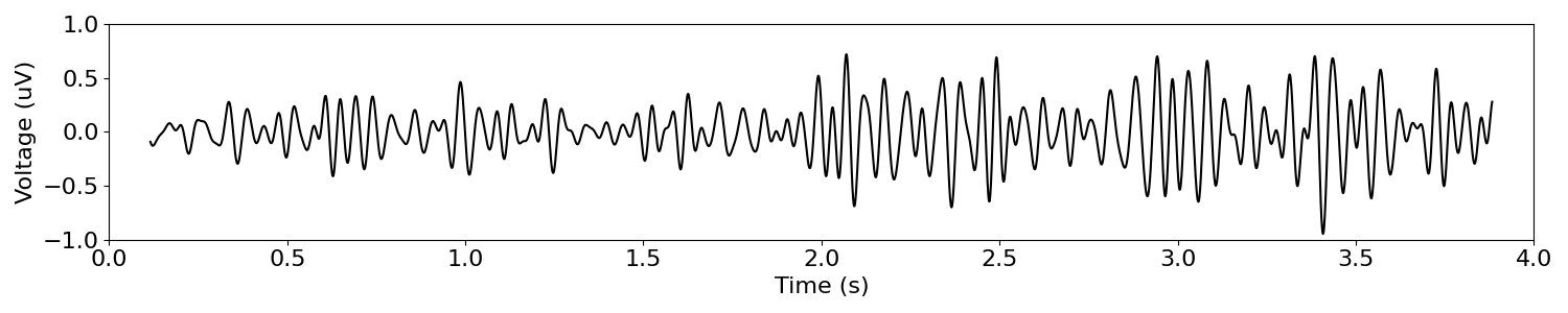
In the above, we can see that this shift in the aperiodic component of the data exhibits as what looks to be change in beta band activity.

We can also examine what this kind of shift looks like in high frequency regions that are sometimes analyzed, like our ‘high-gamma’ frequency band.

# Filter the signal to the current band definition
band_sig = filter_signal(sig_delta_ap, s_rate, 'bandpass', bands.high_gamma)

# Plot the filtered time series
plot_time_series(times, band_sig, xlim=(0, n_seconds), ylim=(-1, 1))

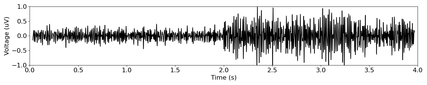
Collectively, we can see that changes in aperiodic properties, that affect all frequencies, can look like band-specific changes when time series are analyzed using narrow-band filters.

If individual bands are filtered and analyzed in isolation, without comparison to either aperiodic measures, or other frequency bands, this kind of analysis could mis-interpret broadband aperiodic changes as oscillatory changes.

Note that in real data, to what extent such aperiodic shifts occur is something of an open question. Within subject changes in aperiodic activity has been observed, and so this remains a possibility that should be considered.

Conclusions

Here we have seen that filtering signals to narrow band signals can return results that reflect periodic activity and dynamics. We therefore suggest that narrow band filtered signals should not be presumed to necessarily reflect periodic activity. In order to ascertain whether narrow band frequency regions reflect periodic and/or aperiodic activity and which aspects are changing in the data, additional analyses, such as parameterizing neural power spectra, are recommended.