Rhythmicity of Time Series

Exploring the rhythmicity of time series and their frequency representations.

Rhythmicity of Time Series

Central to the motivation for parameterizing neural power is the claim that power at a given frequency is not sufficient to claim that there is evidence for rhythmic, or periodic, activity at that frequency.

In this example, we will explore this idea by examining some example signals in the time domain, and their frequency domain representations. We will use these signals to motivate if and when signals should be interpreted as containing periodic activity.

The Fourier Theorem

Stated informally, the Fourier theorem tells us that any time series can be represented as a sum of sinusoids.

This is a powerful and useful theorem, as it means that we can use tools such as the Fourier transform and other similar measures, to compute frequency representations of any time series data.

However, just because a signal can be represented by sinusoids does not mean that any given signal, or any given aspect of a signal, for which a power spectrum can be computed should be conceptualized as being comprised of rhythmic components.

The power spectrum is just a possible representation of the original data, not a descriptive claim of the actual components of the data.

# Import numpy
import numpy as np

# Use NeuroDSP for time series simulations & analyses
from neurodsp import sim
from neurodsp.utils import create_times
from neurodsp.spectral import compute_spectrum_welch
from neurodsp.plts import plot_time_series, plot_power_spectra

# Set random seed, for consistency generating simulated data
sim.set_random_seed(21)

# Simulation Settings
n_seconds = 2
s_rate = 1000

# Compute an array of time values, for plotting, and check length of data
times = create_times(n_seconds, s_rate)
n_points = len(times)

Frequency Representations of Aperiodic Signals

Let’s start with aperiodic signals, and examine how different types of aperiodic signals are represented in the frequency domain.

The Dirac Delta

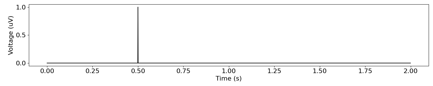
The Dirac delta is arguably the simplest signal, as it’s a signal of all zeros, except for a single value of 1.

# Simulate a delta function
dirac_sig = np.zeros([n_points])
dirac_sig[500] = 1

# Plot the time series of the delta signal
plot_time_series(times, dirac_sig)

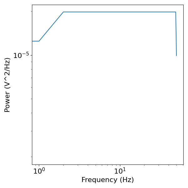
Next, lets compute the frequency representation of the delta function.

# Compute a power spectrum of the Dirac delta
freqs, powers = compute_spectrum_welch(dirac_sig, 100)

# Plot the power spectrum of the Dirac delta
plot_power_spectra(freqs, powers)

Section Conclusions

As we can see above, the power spectrum of the Dirac delta function has power across all frequencies.

This is despite it containing containing a single non-zero value, and thus having no rhythmic properties to it in the time domain.

The Dirac delta example can be taken as a proof of principle that observing power at a particular frequency does not necessarily imply that one should consider that there are any rhythmic properties at that frequency in the original time series.

In this case, and many like it, power across all frequencies is a representation of transient (or aperiodic) activity in the time series. Broadly, when there are transients, or aperiodic components, lots of sinusoids have to be added together in order to represent aperiodic activity out of a basis set of periodic sine waves, and this is why such signals typically look very broadband in the frequency domain.

Colored Noise Signals

Let’s now look at ‘noise’ signals.

In the signals below, we will simulate colored noise signals, in which samples are drawn randomly from noise distributions, with no rhythmic properties.

As we will see, in the power spectrum, these signals exhibit power at all frequencies, with specific patterns of powers across frequencies, which is dependent on the ‘color’ of the noise.

White Noise

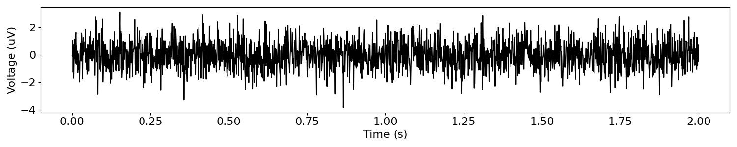
A ‘white noise’ signal is one that is generated with uncorrelated samples drawn from a random distribution. Since each element of the signal is sampled randomly, there is no consistent rhythmic structure in the signal.

# Generate a white noise time series signal
white_sig = np.random.normal(0, 1, n_points)

# Plot the white noise time series
plot_time_series(times, white_sig)

As before, we can compute and visualize the power spectrum of this signal.

# Compute the power spectrum of the white noise signal
freqs, powers = compute_spectrum_welch(white_sig, s_rate)

# Visualize the power spectrum of the white noise signal
plot_power_spectra(freqs, powers)

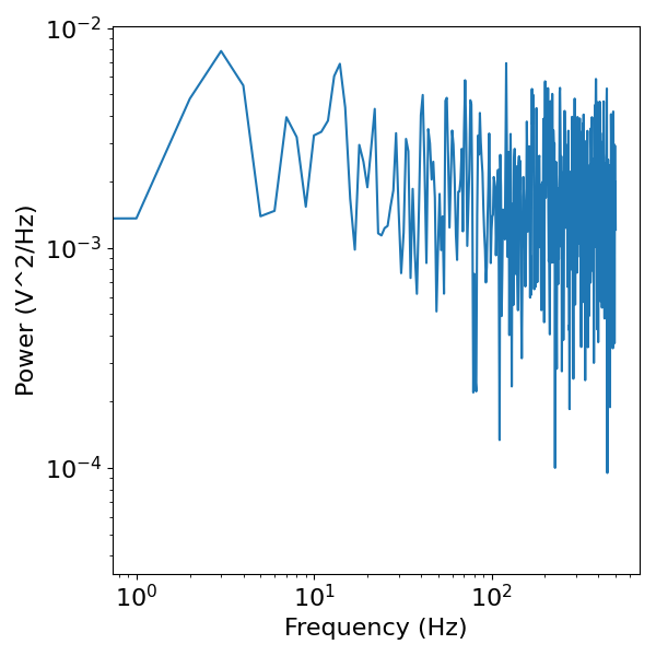
In the frequency representation, we can see that white noise has a flat power spectrum, with equal power across all frequencies. This is the definition of white noise.

This is similar to the delta function, though note that in this case the power across frequencies is representing continuous aperiodic activity, rather than a single transient.

Pink Noise

Other ‘colors’ of noise refer to different patterns of power distributions in the power spectrum.

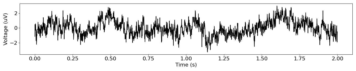
For example, pink noise is a signal where power systematically decreases across frequencies in the power spectrum.

# Generate a pink noise signal
pink_sig = sim.sim_powerlaw(n_seconds, s_rate, exponent=-1)

# Plot the pink noise time series
plot_time_series(times, pink_sig)

# Compute the power spectrum of the pink noise signal
freqs, powers = compute_spectrum_welch(pink_sig, s_rate)

# Visualize the power spectrum of the pink noise signal
plot_power_spectra(freqs, powers)

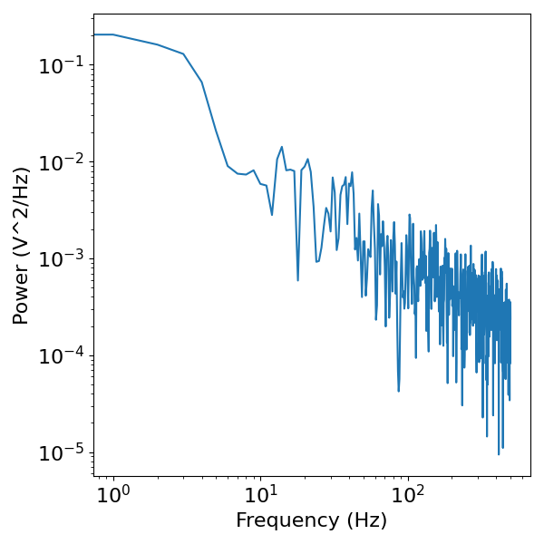
Section Conclusion

The ‘colored noise’ signals above are simulated signals with no rhythmic properties, in the sense that there are no characteristic frequencies or visible rhythms in the data.

Nevertheless, and by definition, in the power spectra of such signals, there is power across all frequencies, with some pattern of power across frequencies.

However, there are no frequencies at which power is different from expected from an aperiodic noise signal. These signals are statistically, by definition, aperiodic.

Frequency Representations of Rhythmic Signals

Next, lets check what frequency representations look like for time series that do have rhythmic activity.

Sinusoidal Signals

There are many different rhythmic signals we could simulate, in terms of different rhythmic shapes, and or temporal properties (such as rhythmic bursts). For this example, we will stick to simulating continuous sinusoidal signals.

# Generate an oscillating signal
osc_sig = sim.sim_oscillation(n_seconds, s_rate, freq=10)

# Plot the oscillating time series
plot_time_series(times, osc_sig)

# Compute the power spectrum of the oscillating signal
freqs, powers = compute_spectrum_welch(osc_sig, s_rate)

# Visualize the power spectrum of the oscillating signal
plot_power_spectra(freqs, powers)

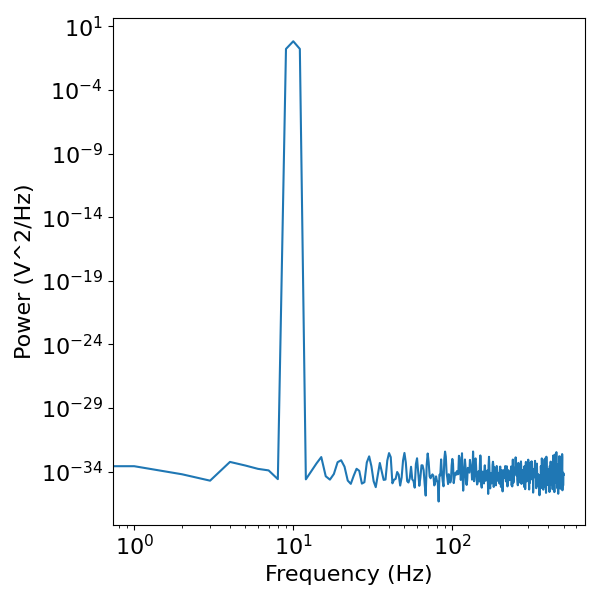
Section Conclusion

When there is rhythmic activity at a particular frequency, this exhibits as a ‘peak’ of power in the frequency domain. This peak indicates high power at a specific frequency, where as the power values at all other frequencies are effectively zero.

Frequency Representations of Complex Signals

Now let’s consider the case whereby one could have a signal comprised of multiple components, for example one or more oscillations combined with an aperiodic component.

Combined Aperiodic & Periodic Signals

To examine this, we will simulate combined signals, comprising both periodic and aperiodic components, and see what the frequency representations look like.

# Define component of a combined signal: an oscillation and an aperiodic component
components = {
    'sim_oscillation' : {'freq' : 10},
    'sim_powerlaw' : {'exponent' : -1}
}

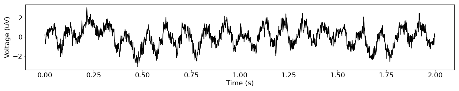
# Generate a combined signal
combined_sig = sim.sim_combined(n_seconds, s_rate, components)

# Plot the combined time series
plot_time_series(times, combined_sig)

# Compute the power spectrum of the combined signal
freqs, powers = compute_spectrum_welch(combined_sig, s_rate)

# Visualize the power spectrum of the combined signal
plot_power_spectra(freqs, powers)

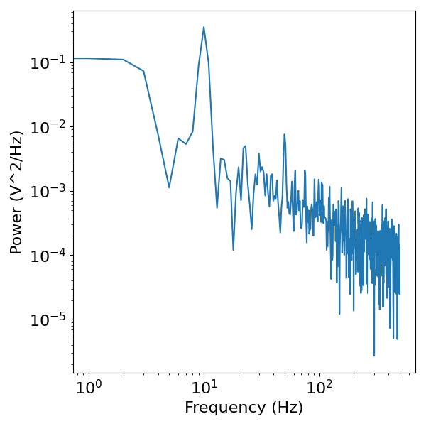
Section Conclusion

In the power spectrum above, we can see that combined signals, with aperiodic & periodic activity reflect elements of both components. The periodic power can be seen as a peak of power over and above the rest of the spectrum, at the frequency of the simulated rhythm. Across all frequencies, we also see the power contributed by the aperiodic component.

Conclusion

In this example, we have seen that, in the frequency domain:

• transients and aperiodic activity exhibit power across all frequencies

• oscillations exhibit specific power, or a ‘peak’, at the frequency of the rhythm

• combined signals display a combination of these properties, with power across all frequencies, and overlying ‘peaks’ at frequencies with periodic activity

Collectively, we have seen cases that motivate that simply having power at a particularly frequency does not imply any rhythmic component at that frequency. Peaks of frequency specific power are associated with rhythmic activity in the time series.

What we have covered here are just a starting point for some properties of time series analysis and digital signal processing. For neural data, these properties alone do not tell us how to interpret neural power spectra. However, here we take them as a starting point that motivate why prominent rhythms in the time series can be measured as peaks in the power spectrum, but that absent a peak, we should not automatically interpret power at any given frequency as necessarily reflecting rhythmic activity.